Contents

Coil currents design study

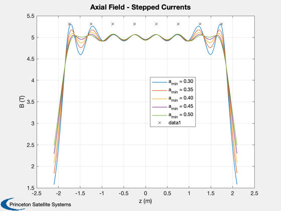
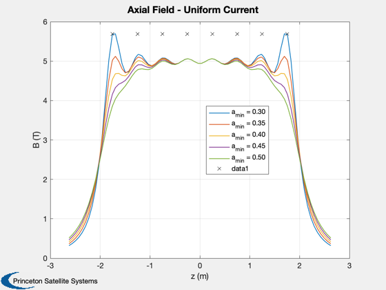
Calculate the radii for an ellipsoidal solenoid and calculate the currents to maintain a desired average field. This is compared to a uniform current in the same coils.

Note: for a 4 m long PFRC, 16 magnets produce a much more uniform field. 8 magnets are more suitable for a 2 m long PFRC.

See also: EllipsoidalSolenoid, ConcentricCoils, PFRCSolenoid

%--------------------------------------------------------------------------
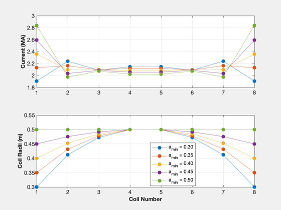
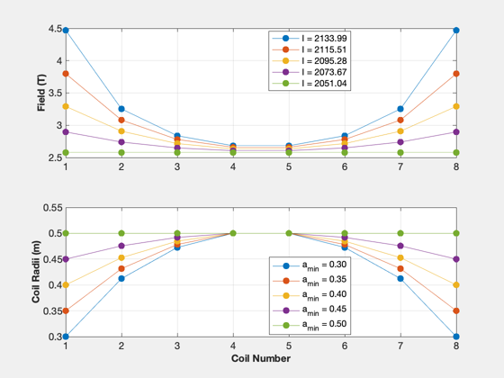
% Copyright (c) 2016 Princeton Satellite Systems, Inc.
% All rights reserved.
%--------------------------------------------------------------------------

% Taper the coil following an ellipsoid and calculate currents to create a
% nearly constant axial field
zC    = [-1.75 -1.25 -0.75 -0.25 0.25 0.75 1.25 1.75];
bAve  = 5;
n     = length(zC);
aMin  = [0.3 0.35 0.4 0.45 0.5];
m     = length(aMin);
b     = zeros(m,500);
i     = zeros(m,n);
a     = zeros(m,n);

s = {};
for k = 1:m
  a(k,:)           	= EllipsoidalSolenoid( aMin(k), 0.5, zC );
  [b(k,:),i(k,:),z]	= ConcentricCoils( zC, bAve, a(k,:) );
  s{k}              = sprintf('a_{min} = %4.2f',aMin(k));
end

ll = {};
IT = [];
B  = [];
for k = 1:m
  a(k,:)  = EllipsoidalSolenoid( aMin(k), 0.5, zC );
  gamma   = 1;
  [IT(k,:),~,~,B(k,:),zs] = PFRCSolenoid(a(k,:),gamma,bAve);
  bm(k,:) = FieldCurrentLoop( a(k,:), IT(k,:), 0 );
  ll{k}   = sprintf('I = %4.2f',IT(k,1)*1e-3);
end

h1 = Plot2D(z,b,'z (m)', 'B (T)', 'Axial Field - Stepped Currents');
legend(s,'location','best')
hold on
plot(zC,max(b(:))*ones(size(zC)),'kx')
h3 = Plot2D(zs,B,'z (m)', 'B (T)', 'Axial Field - Uniform Current');
legend(s,'location','best')
hold on
plot(zC,max(B(:))*ones(size(zC)),'kx')

h2 = NewFig('Coil Radii and Stepped Currents');
subplot(2,1,1)
plot(1:n,i/1e6,'.-','markersize',20);
YLabelS('Current (MA)');
grid on
subplot(2,1,2)
plot(1:n,a,'.-','markersize',20);
grid on
YLabelS('Coil Radii (m)');
XLabelS('Coil Number');
legend(s,'location','best')

h2 = NewFig('Coil Radii and Uniform Current');
subplot(2,1,1)
plot(1:n,bm,'.-','markersize',20);
YLabelS('Field (T)');
grid on
legend(ll,'location','best')
subplot(2,1,2)
plot(1:n,a,'.-','markersize',20);
grid on
YLabelS('Coil Radii (m)');
XLabelS('Coil Number');
legend(s,'location','best')


if 0
  PrintFig(1,4,h1,'CoilB');
  PrintFig(1,4,h2,'CoilAR');
end

DispWithTitle(a','Coil Radius')
DispWithTitle(i','Coil Current')

disp(i)

return

Coil Radius
          0.3         0.35          0.4         0.45          0.5
      0.41231      0.43157      0.45277      0.47566          0.5
      0.47258      0.47828      0.48477      0.49202          0.5
          0.5          0.5          0.5          0.5          0.5
          0.5          0.5          0.5          0.5          0.5
      0.47258      0.47828      0.48477      0.49202          0.5
      0.41231      0.43157      0.45277      0.47566          0.5
          0.3         0.35          0.4         0.45          0.5
Coil Current
   1.9074e+06   2.1318e+06   2.3588e+06   2.5931e+06   2.8375e+06
   2.2397e+06   2.1648e+06   2.0974e+06    2.035e+06   1.9752e+06
   2.0902e+06   2.0964e+06   2.0947e+06   2.0869e+06   2.0744e+06
   2.1477e+06   2.1198e+06     2.09e+06   2.0579e+06   2.0231e+06
   2.1477e+06   2.1198e+06     2.09e+06   2.0579e+06   2.0231e+06
   2.0902e+06   2.0964e+06   2.0947e+06   2.0869e+06   2.0744e+06
   2.2397e+06   2.1648e+06   2.0974e+06    2.035e+06   1.9752e+06
   1.9074e+06   2.1318e+06   2.3588e+06   2.5931e+06   2.8375e+06
  Columns 1 through 6
   1.9074e+06   2.2397e+06   2.0902e+06   2.1477e+06   2.1477e+06   2.0902e+06
   2.1318e+06   2.1648e+06   2.0964e+06   2.1198e+06   2.1198e+06   2.0964e+06
   2.3588e+06   2.0974e+06   2.0947e+06     2.09e+06     2.09e+06   2.0947e+06
   2.5931e+06    2.035e+06   2.0869e+06   2.0579e+06   2.0579e+06   2.0869e+06
   2.8375e+06   1.9752e+06   2.0744e+06   2.0231e+06   2.0231e+06   2.0744e+06
  Columns 7 through 8
   2.2397e+06   1.9074e+06
   2.1648e+06   2.1318e+06
   2.0974e+06   2.3588e+06
    2.035e+06   2.5931e+06
   1.9752e+06   2.8375e+06

Compare to fixed-radii, constant-current array of current loops

This is a 2 m long array

iC = 1.5e6;
aMax  = 0.45;
% Field of a single loop
b1 = MagneticFieldCurrentLoop( iC, aMax, [0;0;0], [1;0;0;0], [0;0;0] )
% Field of the array of loops
zF = [-0.9 -0.64 -0.38 -0.13 0.13 0.38 0.64 0.9];
bS = MagneticFieldCurrentLoop( iC*ones(1,8), aMax*ones(1,8), [zF;zeros(1,8);zeros(1,8)], repmat([1;0;0;0],1,8), [0;0;0] )
% Add the nozzle coils
zz = linspace(-1.5,1.5,40);
z2 = [zz;zeros(size(zz));zeros(size(zz))];
bN = MagneticFieldCurrentLoop( [iC*ones(1,8) 3e6*[1 1]],...
  [aMax*ones(1,8) 0.1*[1 1]], [[zF 1.25 -1.25];zeros(1,10);zeros(1,10)],...
  repmat([1;0;0;0],1,10), z2 );
Plot2D(zz,bN(1,:),'z','Bz','Axial Scan')


%--------------------------------------

Published with MATLAB® R2020a