Contents

Create a compensating coil for the DFD dipole

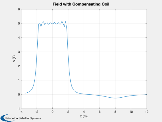
Uses AWG3 wire. The field is computed to see the effect of the compensating coils on the central field of the solenoid.

See also: ConcentricCoils

%--------------------------------------------------------------------------
%   Copyright (c) 2017 Princeton Satellite Systems, Inc.
%   All Rights Reserved.
%--------------------------------------------------------------------------

% The DFD dipole

bAxial  = 5; % T
rCC     = 2; % Radius of compensating coil
zCC     = 8; % Location of compensating coil

% Coil locations
zC      = [-1.75 -1.25 -0.75 -0.25 0.25 0.75 1.25 1.75];

% Coil radii
r       = EllipsoidalSolenoid( 0.35, 0.5, zC ); % Radii

% https://en.wikipedia.org/wiki/American_wire_gauge
% Gauge: AWG3, area is 26.7 mm2
iAWG3   = 115; % Maximum capacity of wire (A)
rho     = 0.6465e-3; % ohms/m
linear  = 8.9*26.7*1e-2; % linear density copper (g/cm)

% superconductors - should specify which material at what temp
iHTS = 500;
linearHTS = 0.085; % g/cm

% Compute the coil currents
[~, i]	= ConcentricCoils( zC, bAxial, r )

% Compute the dipoles and compensating coil
mDFD    = pi*sum(r.^2.*i);
zC      = [zC zCC]; % Z location
r       = [r  rCC]; % Radii
z       = linspace(2*zC(1),1.5*zC(end));
iCC     = mDFD/(pi*rCC^2);
n       = iCC/iAWG3;
l       = 2*pi*rCC*n; % total length of wire
power   = iAWG3^2*rho*l;
mass    = linear*l*0.1; % mass of copper (kg)
massHTS = iCC/iHTS*2*pi*rCC*linearHTS*0.1

k       = 1;
s = {};
s{k,1}	= 'Mass';               s{k,2}= sprintf('%12.2f kg',mass);  k = k + 1;
s{k,1}	= 'Power consumption';  s{k,2}= sprintf('%12.2f kW',power/1000);  k = k + 1;
s{k,1}	= 'Current';            s{k,2}= sprintf('%12.2f MA',iCC/1e6);     k = k + 1;
s{k,1}	= 'Number of turns';    s{k,2}= sprintf('%12.0f',n);              k = k + 1;
s{k,1}	= 'Radius';             s{k,2}= sprintf('%12.2f m',rCC);          k = k + 1;
s{k,1}	= 'DFD B Field';        s{k,2}= sprintf('%12.2f T',bAxial);

DisplayLatexTable(s)

i       = [i -iCC];
b       = Field(i,r,zC,z);

Plot2D(z,b,'z (m)', 'b (T)', 'Field with Compensating Coil');

i =
  Columns 1 through 6
   2.1318e+06   2.1648e+06   2.0964e+06   2.1198e+06   2.1198e+06   2.0964e+06
  Columns 7 through 8
   2.1648e+06   2.1318e+06
massHTS =
       178.79
             Mass     21731.80 kg 
Power consumption       781.91 kW 
          Current         0.84 MA 
  Number of turns            7278 
           Radius          2.00 m 
      DFD B Field          5.00 T 

Axial field computation

function b = Field( i, a, d, z )

mu0   = 4e-7*pi;
a2    = a.^2;
f     = mu0*i.*a2/2;
b     = zeros(1,length(z));

for k = 1:length(d)
  b = b + f(k)./((z-d(k)).^2 + a2(k)).^1.5;
end

end


%--------------------------------------

Published with MATLAB® R2020a