Contents

Fuel mix analysis demo creating contour plots

Uses a fixed electron temperature for all computations.

- to make the colormaps uniform: caxis([0.2 50]) - to lighten the colors: brighten(0.5)

Reference: Carpenter 1999, Figure 4

%--------------------------------------------------------------------------
% See also: PowerDHe3, Synchrotron
%--------------------------------------------------------------------------

%--------------------------------------------------------------------------
%	Copyright (c) 2018 Princeton Satellite Systems, Inc. All rights reserved.
%--------------------------------------------------------------------------

ratios = logspace(-1.6,0.5);
temps = linspace(40,140);

d = PowerDHe3;

ne = 4e20;
zI = [1 2];
b = 5;

d.tE   = 30;   % electron temp
d.fD   = 1;    % as low as 0.25
d.fT   = 1;

pF = zeros(length(temps),length(ratios));
pN = [];
pB = [];
pS = [];

Model with equal temperatures, full T; electron temp is 0.9 Ti

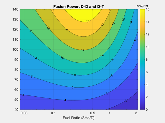
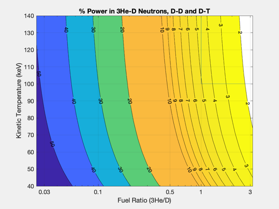
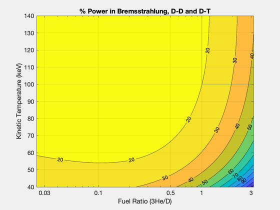
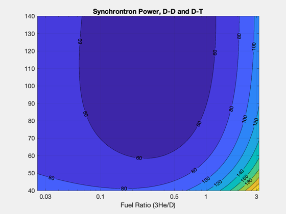
d.fD   = 1;    % as low as 0.25
d.fT   = 1;
for k=1:length(ratios)
  % calculate ion densities from electron density assuming fuel ratio
  den = 1 + 2*ratios(k);
  density = 1/den*ne;
  d.nD = density;
  d.nHe3 = density*ratios(k);
  for j = 1:length(temps)
    d.tHe3 = temps(j);   % potentially uo to 140 keV
    d.tD   = temps(j);   % potentially 70 keV
    d.tE   = 0.9*temps(j);

    % these are powers in MW per cubic meter
    [pF(j,k), pN(j,k), pB(j,k), nNd, nNt] = PowerDHe3( d );
    pS(j,k) = Synchrotron( [d.nD d.nHe3], zI, b, d.tE );
  end
end

MakePlots( ratios, temps, pN, pB, pS, pF,...
  [2 3 4 5 6 7 8 9 10 20 30 40 50], 'D-D and D-T' )
drawnow;

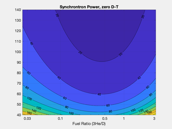
Model with equal temperatures, all T removed

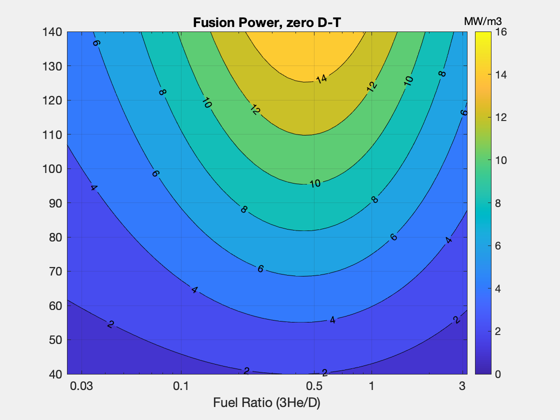
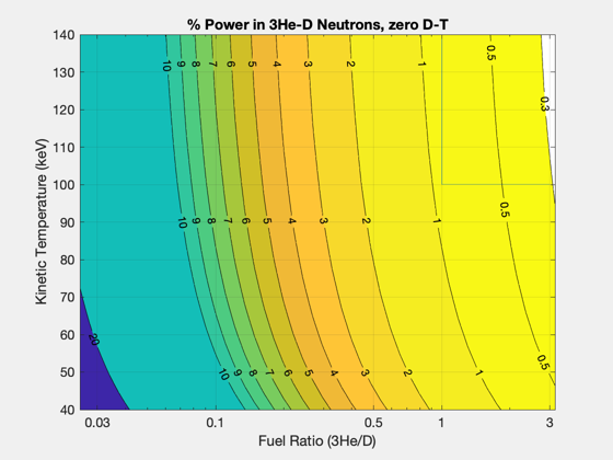
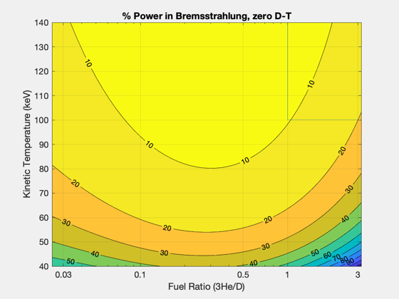
d.fD   = 1;    % as low as 0.25
d.fT   = 0;
d.tE   = 30;   % electron temp
pF = [];
pN = [];
pB = [];
pS = [];
for k=1:length(ratios)
  % calculate ion densities from electron density assuming fuel ratio
  den = 1 + 2*ratios(k);
  density = 1/den*ne;
  d.nD = density;
  d.nHe3 = density*ratios(k);
  for j = 1:length(temps)
    d.tHe3 = temps(j);   % potentially uo to 140 keV
    d.tD   = temps(j);   % potentially 70 keV

    % these are powers in MW per cubic meter
    [pF(j,k), pN(j,k), pB(j,k), nNd, nNt] = PowerDHe3( d );
    pS(j,k) = Synchrotron( [d.nD d.nHe3], zI, b, d.tE );
  end
end

MakePlots( ratios, temps, pN, pB, pS, pF,...
  [0.3 0.5 1 2 3 4 5 6 7 8 9 10 20], 'zero D-T' )
drawnow

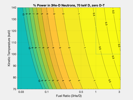
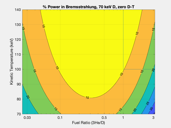
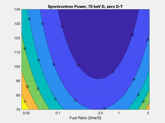
Model with different temperatures

temps2 = linspace(70,140);
d.fD   = 1;    % as low as 0.25
d.fT   = 0;
d.tD   = 70;   % potentially 70 keV
d.tE   = 30;   % electron temp
pF = [];
pN = [];
pB = [];
pS = [];
for k=1:length(ratios)
  % calculate ion densities from electron density assuming fuel ratio
  den = 1 + 2*ratios(k);
  density = 1/den*ne;
  d.nD = density;
  d.nHe3 = density*ratios(k);
  for j = 1:length(temps2)
    d.tHe3 = temps2(j);   % potentially uo to 140 keV

    % these are powers in MW per cubic meter
    [pF(j,k), pN(j,k), pB(j,k), nNd, nNt] = PowerDHe3( d );
    pS(j,k) = Synchrotron( [d.nD d.nHe3], zI, b, d.tE );
  end
end

MakePlots( ratios, temps2, pN, pB, pS, pF,...
  [0.1 0.2 0.3 0.5 1 2 3 4 5 6 7 8 9 10 20], '70 keV D, zero D-T' )

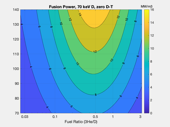
Finished

Figui;


function MakePlots( ratioPlot, tempPlot, pN, pB, pS, pF, N, str )

NewFig('Neutron Power')
[c,h] = contourf(ratioPlot,tempPlot,pN./pF*100,N);
clabel(c,h);
set(gca,'xscale','log')
grid on;
title(['% Power in 3He-D Neutrons, ' str])
xlabel('Fuel Ratio (3He/D)')
ylabel('Kinetic Temperature (keV)')
set(gca,'xtick',[0.03 0.1 0.5 1 3])
set(gcf,'colormap',flipud(parula))
line([1 1],[100 140])
line([1 3],[100 100])

NewFig('Bremsstrahlung Power')
[c,h] = contourf(ratioPlot,tempPlot,pB./pF*100);
clabel(c,h);
set(gca,'xscale','log')
grid on;
title(['% Power in Bremsstrahlung, ' str])
xlabel('Fuel Ratio (3He/D)')
ylabel('Kinetic Temperature (keV)')
set(gca,'xtick',[0.03 0.1 0.5 1 3])
set(gcf,'colormap',flipud(parula))
line([1 1],[100 140])
line([1 3],[100 100])

NewFig('% Power in Synchrotron (10% volume)')
[c,h] = contourf(ratioPlot,tempPlot,0.1*pS./pF*100);
clabel(c,h);
set(gca,'xscale','log')
set(gca,'xtick',[0.03 0.1 0.5 1 3])
grid on;
xlabel('Fuel Ratio (3He/D)')
title(['Synchrontron Power, ' str])

NewFig('Total Fusion Power')
[c,h] = contourf(ratioPlot,tempPlot,pF);
clabel(c,h);
set(gca,'xscale','log')
set(gca,'xtick',[0.03 0.1 0.5 1 3])
grid on;
xlabel('Fuel Ratio (3He/D)')
title(['Fusion Power, ' str])
caxis([0 16]) % Note: will change if tE, etc are changed!!
cb = colorbar;
cb.Title.String = 'MW/m3';

end


%--------------------------------------

Published with MATLAB® R2020a