Contents
Fusion Reactor Design demo
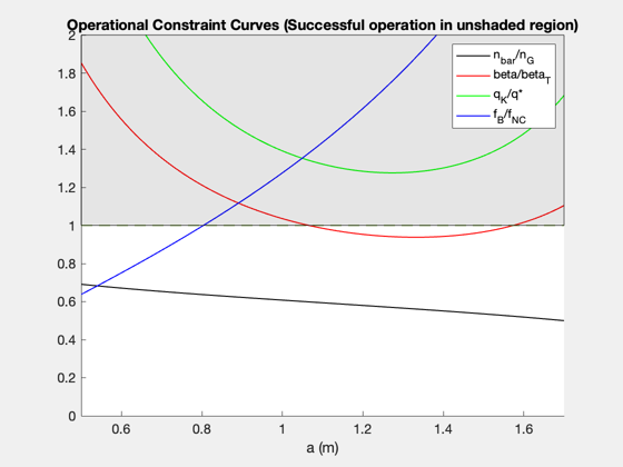
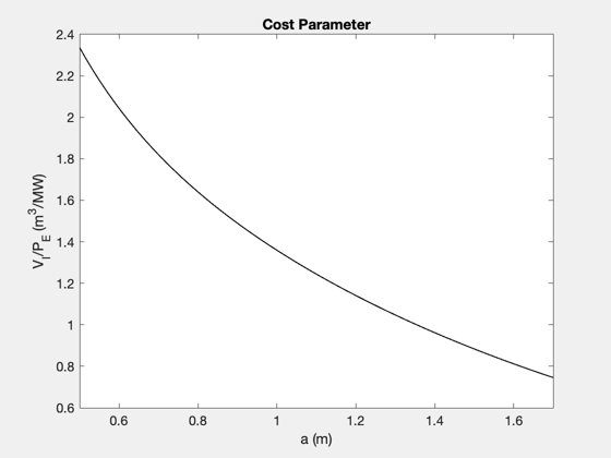
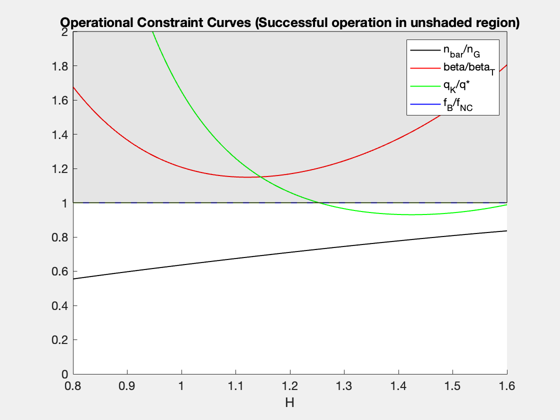
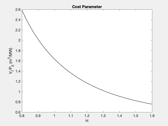
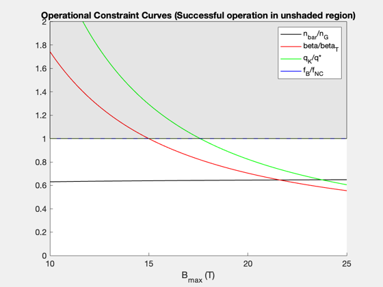
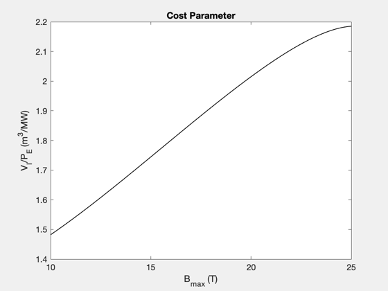
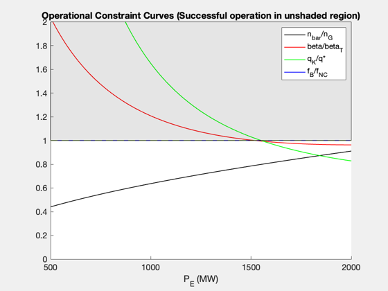
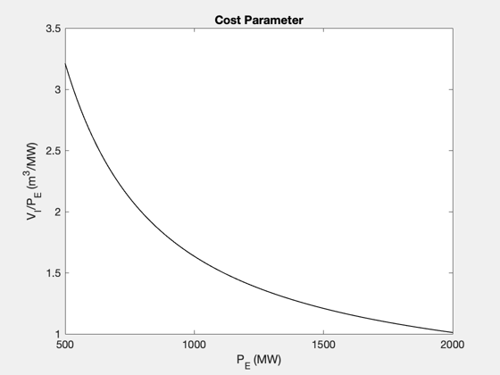
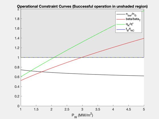
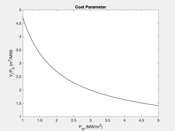
Reproduce the figures/tables from the original reference paper. Each time you call the function you specify the mode, which is the dependent variable that you're interested in. ------------------------------------------------------------------------ Reference: Freidberg, Mangiarotti, and Minervini, "Designing a tokamak fusion reactor--How does plasma physics fit in?" Physics of Plasmas 22, 070901 (2015). ------------------------------------------------------------------------ See also FusionReactorDesign ------------------------------------------------------------------------
%--------------------------------------------------------------------------
%   Copyright (c) 2022 Princeton Satellite Systems, Inc.
%   All rights reserved. Since version 2022.1
%--------------------------------------------------------------------------
Set up input data structures for each variable sweep (a,H,B_max,P_E,P_W)
% Data structure for the case that the input variable is the plasma minor
% radius, a. Note that the default data structure does not need to be
% altered in this case, since the default data was chosen to reproduce
% the first results figure, Figure 5, in the reference.
d_a = FusionReactorDesign;

% Compute plots ("curves") and tables ("parameters") from the reference
d_a = FusionReactorDesign(d_a,'a');

% Data structure for the case that the input variable is the H-mode
% enhancement factor, H
d_H = FusionReactorDesign;
d_H.B_max = 13;
d_H.H = 1.26;
d_H.P_E = 1000; % electric power output [MW]
d_H.P_W = 4; % max neutron wall loading [MW/m2]
d_H.a = 1.26;

% Compute plots and table from the reference
d_H = FusionReactorDesign(d_H,'H');

% Data structure for the case that the input variable is the maximum
% magnetic field at the coil, B_max.
d_Bmax = FusionReactorDesign;
d_Bmax.B_max = 17.6;
d_Bmax.H = 1;
d_Bmax.P_E = 1000; % electric power output [MW]
d_Bmax.P_W = 4; % max neutron wall loading [MW/m2]
d_Bmax.a = 0.97;

% We will also specify the minimum, maximum, and length of the input vector
% in this case.
pmin = 10;
pmax = 25;
n    = 100;

% Compute plots and table from the reference
d_Bmax = FusionReactorDesign(d_Bmax,'B_max',pmin,pmax,n);

% Data structure for the case that the input variable is the electric power
% output, P_E
d_PE = FusionReactorDesign;
d_PE.B_max = 13;
d_PE.H = 1;
d_PE.P_E = 1554; % electric power output [MW]
d_PE.P_W = 4; % max neutron wall loading [MW/m2]
d_PE.a = 1.44;

% Compute plots and table from the reference
d_PE = FusionReactorDesign(d_PE,'P_E');

% Data structure for the case that the input variable is maximum input wall
% loading, P_W
d_PW = FusionReactorDesign;
d_PW.B_max = 13;
d_PW.H = 1;
d_PW.P_E = 1000; % electric power output [MW]
d_PW.P_W = 2.1; % max neutron wall loading [MW/m2]
d_PW.a = 1.35;

% Compute plots and table from the reference
d_PW = FusionReactorDesign(d_PW,'P_W');

% Display output tables (these correspond to the various columns, in order,
% in Table III of the reference)
disp(d_a.parameters)
disp(d_H.parameters)
disp(d_Bmax.parameters)
disp(d_PE.parameters)
disp(d_PW.parameters)


%--------------------------------------

% $Id: 0c42080762886b3751bf661818ff650348f32380 $
        Quantity         Output
    _________________    _______

    {'Bmax(T)'      }         13
    {'H'            }          1
    {'PE(MW)'       }       1000
    {'PW(MW/m^2)'   }          4
    {'VI/PW(m^3/MW)'}     1.0155
    {'Q||(MW-T/m)'  }     498.85
    {'B0(T)'        }     6.8768
    {'a(m)'         }       1.34
    {'c(m)'         }    0.97045
    {'R0(m)'        }     5.3849
    {'R0/a'         }     4.0186
    {'p(atm)'       }     7.5459
    {'n(10^20 m^-3)'}     1.4203
    {'n/nG'         }     0.5604
    {'tauE(s)'      }    0.94747
    {'I(MA)'        }     14.219
    {'beta(%)'      }     4.0635
    {'beta/betaT'   }    0.93794
    {'qstar'        }     1.5598
    {'qK/qstar'     }     1.2822
    {'fB'           }    0.83916
    {'fB/fNC'       }     1.8927

        Quantity         Output
    _________________    _______

    {'Bmax(T)'      }         13
    {'H'            }       1.26
    {'PE(MW)'       }       1000
    {'PW(MW/m^2)'   }          4
    {'VI/PW(m^3/MW)'}     1.0845
    {'Q||(MW-T/m)'  }      506.2
    {'B0(T)'        }     7.4045
    {'a(m)'         }       1.26
    {'c(m)'         }    0.98031
    {'R0(m)'        }     5.7139
    {'R0/a'         }     4.5349
    {'p(atm)'       }     7.7731
    {'n(10^20 m^-3)'}      1.463
    {'n/nG'         }    0.72878
    {'tauE(s)'      }    0.91978
    {'I(MA)'        }     10.003
    {'beta(%)'      }     3.6104
    {'beta/betaT'   }      1.202
    {'qstar'        }     1.9982
    {'qK/qstar'     }     1.0009
    {'fB'           }    0.77237
    {'fB/fNC'       }          1

        Quantity         Output
    _________________    _______

    {'Bmax(T)'      }       17.6
    {'H'            }          1
    {'PE(MW)'       }       1000
    {'PW(MW/m^2)'   }          4
    {'VI/PW(m^3/MW)'}     1.8877
    {'Q||(MW-T/m)'  }     654.47
    {'B0(T)'        }     12.442
    {'a(m)'         }       0.97
    {'c(m)'         }     1.6387
    {'R0(m)'        }     7.4262
    {'R0/a'         }     7.6559
    {'p(atm)'       }     8.8615
    {'n(10^20 m^-3)'}     1.6679
    {'n/nG'         }    0.64247
    {'tauE(s)'      }     0.8068
    {'I(MA)'        }     7.6584
    {'beta(%)'      }     1.4577
    {'beta/betaT'   }     0.8196
    {'qstar'        }     1.9978
    {'qK/qstar'     }     1.0011
    {'fB'           }     0.6843
    {'fB/fNC'       }          1

        Quantity         Output
    _________________    _______

    {'Bmax(T)'      }         13
    {'H'            }          1
    {'PE(MW)'       }       1554
    {'PW(MW/m^2)'   }          4
    {'VI/PW(m^3/MW)'}     1.1785
    {'Q||(MW-T/m)'  }     668.51
    {'B0(T)'        }     8.5718
    {'a(m)'         }       1.44
    {'c(m)'         }     1.0666
    {'R0(m)'        }     7.7407
    {'R0/a'         }     5.3755
    {'p(atm)'       }     7.2776
    {'n(10^20 m^-3)'}     1.3698
    {'n/nG'         }     0.7971
    {'tauE(s)'      }     0.9824
    {'I(MA)'        }     11.144
    {'beta(%)'      }     2.5223
    {'beta/betaT'   }    0.99552
    {'qstar'        }     1.9948
    {'qK/qstar'     }     1.0026
    {'fB'           }    0.69587
    {'fB/fNC'       }          1

        Quantity         Output
    _________________    _______

    {'Bmax(T)'      }         13
    {'H'            }          1
    {'PE(MW)'       }       1000
    {'PW(MW/m^2)'   }        2.1
    {'VI/PW(m^3/MW)'}     2.5987
    {'Q||(MW-T/m)'  }     373.58
    {'B0(T)'        }     9.7459
    {'a(m)'         }       1.35
    {'c(m)'         }     1.1202
    {'R0(m)'        }     10.191
    {'R0/a'         }     7.5487
    {'p(atm)'       }     5.4263
    {'n(10^20 m^-3)'}     1.0213
    {'n/nG'         }    0.68694
    {'tauE(s)'      }     1.3176
    {'I(MA)'        }      8.524
    {'beta(%)'      }     1.4548
    {'beta/betaT'   }    0.80252
    {'qstar'        }     1.9912
    {'qK/qstar'     }     1.0044
    {'fB'           }    0.66258
    {'fB/fNC'       }          1