Simulation of Automobile Suspension

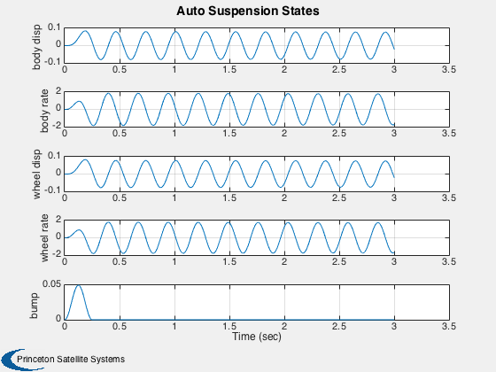
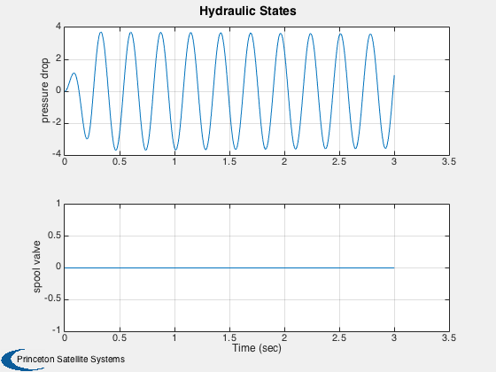
Simulates a quarter automobile model for the suspension with a hydraulic actuator. The automobile parameters and actuator parameters are defined and a bump disturbance is considered. The natural motion is simulated for three seconds (no control) and the results for the auto suspension and hydraulic states are displayed.

Since version 1.
-------------------------------------------------------------------------
Reference: Lin, J. and I. Kanellakopoulos (1997.) Nonlinear Design of
           Active Suspensions. IEEE Control Systems Magazine,
           June 1997. pp. 45-59
-------------------------------------------------------------------------
See also:  RHSAutoSuspension, DBump, TimeGUI, Plot2D
-------------------------------------------------------------------------

Global for the time GUI
Automobile parameters
Hydraulic actuator parameters
Bump disturbance
Control
State
The control sampling period and the simulation integration time step
Number of sim steps
Plotting arrays
Time statistics function
Initialize the time display
Run the simulation
Plot results

%--------------------------------------------------------------------------
%   Copyright (c) 2001 Princeton Satellite Systems, Inc.
%   All rights reserved.
%--------------------------------------------------------------------------

Global for the time GUI

Creates a global variable for the time GUI, which displays the time remaining and estimated completion of a simulation. It computes the time left to go in the simulation, the predicted finish time and the ratio of simulation time to real time. -------------------------------------------------------------------------

global simulationAction
simulationAction = ' ';

Automobile parameters

SI units. ----------------------

d.mB    =    290; % Body mass (kg)
d.mUS   =     59; % Wheel mass (kg)
d.kA    =  16812; % Spring constant (N/m)
d.cA    =   1000; % Damping constant (N/(m/sec))
d.kT    = 190000; % Tire spring constant (N/m)

Warning: Struct field assignment overwrites a value with class "double". See
MATLAB R14SP2 Release Notes, Assigning Nonstructure Variables As Structures
Displays Warning, for details.

Hydraulic actuator parameters

------------------------------

d.alpha = 4.515e13; % N/m^5
d.beta  = 1; % alpha times piston leakage coefficient (1/s)
d.gamma = 1.545e9; % N/(m^5/2 kg^1/2)
d.tau   = 1/30; % Spool valve time constant (s)
d.pS    = 10342500; % Supply pressure (Pa)
d.a     = 3.35e-4; % Piston area (m^2)

Bump disturbance

-----------------

d.aBump = 0.025; % Bump amplitude (m)
d.wBump = 8*pi;  % Bump frequency (rad/sec)

Control

--------

d.u     = 0;

State

Form: [car body displacement;... car body rate;... wheel displacement;... wheel rate;... pressure drop across the piston;... spool valve displacement] ------------------------------------------

x           = [0;0;0;0;0;0];
t           = 0;

The control sampling period and the simulation integration time step

---------------------------------------------------------------------

dT          = 1;

Number of sim steps

--------------------

tEnd        = 3;
nSim        = 2000;
dT          = tEnd/(nSim-1);

Plotting arrays

----------------

tPlot      = zeros(1,nSim);
xPlot      = zeros(7,nSim);

Time statistics function

-------------------------

tToGoMem      = [];
ratioRealTime = 0;

Initialize the time display

----------------------------

tToGoMem.lastJD        = 0;
tToGoMem.lastStepsDone = 0;
tToGoMem.kAve          = 0;
ratioRealTime          = 0;
[ ratioRealTime, tToGoMem ] =  TimeGUI( nSim, 0, tToGoMem, 0, dT,...
    'Auto Suspension States' );

a = Jacobian( 'RHSAutoSuspension', x, t, d )

a =
            0            1            0            0            0            0
      -57.972      -3.4483       57.972       3.4483       11.552            0
            0            0            0            1            0            0
       284.95       16.949      -3505.3      -16.949       -56.78            0
            0      -1512.5            0       1512.5           -1   4.9687e+05
            0            0            0            0            0          -30

Run the simulation

-------------------

for k = 1:nSim

  % Display the status message
  % --------------------------
  [ ratioRealTime, tToGoMem ] = TimeGUI(nSim,k,tToGoMem,ratioRealTime,dT);

  x           = RK4( 'RHSAutoSuspension', x, dT, t, d );
  t           = t + dT;
  tPlot(k)    = t;
  xPlot(:,k)  = [x;DBump( t, d )];

  % Time control
  % ------------
  switch simulationAction
    case 'pause'
      pause
      simulationAction = ' ';
    case 'stop'
      return;
    case 'plot'
      break;
  end

end

TimeGUI( 'close' )

Plot results

This shows open loop results with the hydraulic actuator. The hydraulic actuator effectively dedamps the system. -------------------------------------------------------------------------

j     = 1:k;
tPlot = tPlot(j);

yL    = strvcat(' body disp',...
                ' body rate',...
                ' wheel disp',...
                ' wheel rate',...
                'pressure drop',...
                ' spool valve',...
				'   bump');

k1 = [1:4 7];
k2 = 5:6;
Plot2D( tPlot, xPlot(k1 ,j),'Time (sec)',yL(k1,:),'Auto Suspension States')
Plot2D( tPlot, xPlot(k2 ,j),'Time (sec)',yL(k2,:),'Hydraulic States')

%--------------------------------------
% PSS internal file version information
%--------------------------------------