Tokamak Plasma Vertical Control
Simulates a model of the vertical position of an elongated plasma in a Tokamak. The vertical position is unstable and can be represented by one unstable mode and one stable mode and a time delay. Two major disturbances are due to the thyristor power supplies and the Edge Localized Modes (ELM).
Since version 1.
-------------------------------------------------------------------------
Reference: Scibile, L. and B. Kouvaritakis (2001.) "A Discrete Adaptive
           Near-Time Optimum Control for the Plasma Vertical Position
           in a Tokamak." IEEE Transactions on Control System
           Technology. Vol. 9, No. 1, January 2001.
-------------------------------------------------------------------------
See also:    RHSTPVC, SSTokamak, ELM, getabcd, TimeGUI, Plot2D
-------------------------------------------------------------------------
Contents
%--------------------------------------------------------------------------
%   Copyright (c) 2001 Princeton Satellite Systems, Inc.
%   All rights reserved.
%--------------------------------------------------------------------------
Constants. See HPH.m or FPH.m for definitions
----------------------------------------------
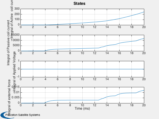
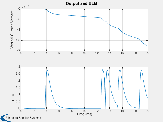
d.rAA                = 35.0e-3;   % Active coil resistance (Ohm)
d.rVV                =  2.56e-3;  % Passive coil resistance(Ohm)
d.lAV                =  0.432e-3; % Active-passive coil mutual inductance (H)
d.lAA                = 42.5e-3;   % Active coil self-inductance (H)
d.lVV                =  0.012e-3; % Passive coil self-inductance (H)
d.lAP                = 115.2e-6;  % Mutual change inductance between the
                                  % active coils and plasma displacement (H/m)
d.lVP                =   3.2e-6;  % Mutual change inductance between the
                                  % passive coils and plasma displacement(H/m)
d.aPP                =   0.4e-6;  % Normalized destabilizing force
                                  % 0.4 to 0.6 e-6 H/m^2
d.g                  = SSTokamak( d ); % Generates a statespace model of a
                                       % tokamak. The output is the
                                       % vertical current moment of the
                                       % plasma current centroid. This
                                       % system is unstable.

% Extract the a,b,c and d matrices from g
%----------------------------------------
[d.a, d.b, d.c, d.d] = getabcd( d.g );
d.fP                 = 0;
d.d600               = 0;
d.tau1ELM            = 6.0e-4;    % Time constant 1
d.tau2ELM            = 1.7e-4;    % Time constant 2
d.kELM               = 6.5;       % Gain
d.tRepELM            = 48e-3;     % Time (s)
d.nDelay             = 3;
d.iP                 = 7e6;
The control sampling period and the simulation integration time step
---------------------------------------------------------------------
dT = .01/100;
Number of sim steps
--------------------
nSim        = 200;
tEnd        = nSim*dT;
tRepELM     = 0;
Plotting arrays
----------------
tPlot      = zeros(1,nSim);
xPlot      = zeros(6,nSim);

% Stack for the delay
%--------------------
delayStack = zeros(1,d.nDelay);
Initial conditions
-------------------
x           = [0;0;0;0];
t           = 0;
tELM        = 20e-3*rand;
v           = 0;
Run the simulation
See ELM.m which is a that gives you the disturbance in a Tokamak plasma due to edge localized modes (ELMs). Also see RHSTPVC.m which simulates a model of the vertical position of a plasma in a Tokamak. -------------------------------------------------------------------------
for k = 1:nSim

  % Simulate the delay
  %-------------------
  delayStack(end)       = v + d.d600*sin(2*pi*600*t);
  delayStack(1:(end-1)) = delayStack(2:end);
  d.v                   = delayStack(1);
  d.eLM                 = ELM( d.tau1ELM, d.tau2ELM, d.kELM, tELM );
  tELM                  = tELM + dT;
  if( t > tRepELM + rand*d.tRepELM )
	 tELM      = 0;
	 tRepELM   = t;
  end

  x           = RK4( 'RHSTPVC', x, dT, t, d );
  t           = t + dT;
  tPlot(k)    = t;
  xPlot(:,k)  = [x;d.c*x + d.d*[d.v;d.fP];d.eLM];

end
Plot results
Open loop results are displayed. --------------------------------
j     = 1:k;
tPlot = tPlot(j)*1000;
yL    = get( d.g, 'states' );
yL2   = { get( d.g, 'outputs' ), 'ELM' };
Plot2D( tPlot, xPlot(1:4,j),'Time (ms)',yL,'States')
Plot2D( tPlot, xPlot(5:6,j),'Time (ms)',yL2,'Output and ELM')

%--------------------------------------
% PSS internal file version information
%--------------------------------------