Simulation for pH process
Simulates a simple model of a pH process. The process consists of an acid (HNO3) stream, buffer (NaHCO3) stream, and base (NaOH) stream that are mixed in a stirred tank. The chemical equilibria is modeled by introducing two reaction invariants for each inlet stream. fzero is used to solve the equations for the PH sensor.
Since version 1.
-------------------------------------------------------------------------
Reference:   List references if applicable
-------------------------------------------------------------------------
See also:    RHSpH, HpH, TimeGUI, Plot2D
-------------------------------------------------------------------------
Contents
%--------------------------------------------------------------------------
%   Copyright (c) 2001 Princeton Satellite Systems, Inc.
%   All rights reserved.
%--------------------------------------------------------------------------
Global for the time GUI
Creates a global variable for the time GUI, which displays the time remaining and estimated completion of a simulation. It computes the time left to go in the simulation, the predicted finish time and the ratio of simulation time to real time. -------------------------------------------------------------------------
global simulationAction
simulationAction = ' ';
Constants
         +        -         -         =
 wAi = [H ]i - [OH ]i - [HCO3]i - 2[CO3]i
                      -         =
 wBi = [H2CO3]i + [HCO3]i + 2[CO3]i
%---------------------------------------------- d.wA1 = 0.003; % Reaction invariant for species A in the acid % stream (M) d.wA2 = -0.03; % Reaction invariant for species A in the buffer % stream(M) d.wA3 = -3.05e-3; % Reaction invariant for species A in the base % stream(M) d.wB1 = 0.0; % Reaction invariant for species B in the effluent % stream(M) d.wB2 = 0.03; % Reaction invariant for species B in the acid % stream(M) d.wB3 = 5.0e-5; % Reaction invariant for species B in the buffer % stream(M) d.pK1 = log10(4.47e-7); % Base 10 log of equilibrium constant d.pK2 = log10(5.62e-11); % Base 10 log of equilibrium constant d.a = 207; % Crossectional area of the mixing tank (cm^2) d.cV = 1; % Valve coefficient d.n = 0.607; % Valve exponent d.z = 11.5; % Vertical distance between bottom of tank and % outlet of effluent (cm) d.q1 = 16.6; % Volumetric flow of HNO3 (ml/s) d.q2 = 15.6; % Volumetric flow of NaHCO3 (ml/s) d.q3 = 0.55; % Volumetric flow of NaOH (ml/s) -used as control wA4 = -4.32e-4; % Reaction invariant for species A in the effluent % stream(M) wB4 = 5.28e-4; % Reaction invariant for species B in the base % stream(M) h = 14.0;
Initial conditions
-------------------
x           = [wA4;wB4;h];
t           = 0;
The control sampling period and the simulation integration time step
---------------------------------------------------------------------
dT = 5/100;
Number of sim steps
--------------------
nSim        = 1000;
tEnd        = nSim*dT;
Plotting arrays
----------------
tPlot      = zeros(1,nSim);
xPlot      = zeros(4,nSim);
Time statistics function
-------------------------
tToGoMem = [];
Initialize the time display
----------------------------
tToGoMem.lastJD        = 0;
tToGoMem.lastStepsDone = 0;
tToGoMem.kAve          = 0;
[ratioRealTime, tToGoMem] = TimeGUI( nSim, 0, tToGoMem, 0, dT, 'pH Simulation' );
Run the simulation
-------------------
for k = 1:nSim

  % Display the status message
  %---------------------------
  [ ratioRealTime, tToGoMem ] = TimeGUI(nSim,k,tToGoMem,ratioRealTime,dT);

  % Integrate one step
  %-------------------
  x           = RK4( 'RHSpH', x, dT, t, d );
  t           = t + dT;
  tPlot(k)    = t;

  % Solve for the nonlinear sensor output
  %--------------------------------------
  y           = fzero( 'HpH', 0, [], x, d );
  xPlot(:,k)  = [x;y];

  % Time control
  %-------------
  switch simulationAction
    case 'pause'
      pause
      simulationAction = ' ';
    case 'stop'
      return;
    case 'plot'
      break;
  end

end

TimeGUI( 'close' )
Plot results
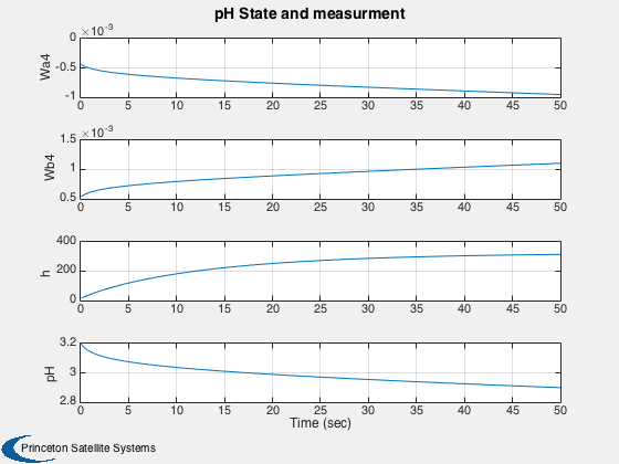
Open loop response.
%--------------------
j     = 1:k;
tPlot = tPlot(j);
xPlot = xPlot(:,j);

Plot2D( tPlot, xPlot,'Time (sec)',{'Wa4' 'Wb4' 'h' 'pH'},'pH State and measurment')

%--------------------------------------
% PSS internal file version information
%--------------------------------------