Demonstrate the ABC machine.
This simulation demonstrates speed control.
------------------------------------------------------------------------
See also Plot2D, TimeLabl, RK4
------------------------------------------------------------------------
Contents
%--------------------------------------------------------------------------
%	Copyright (c) 2009 Princeton Satellite Systems, Inc.
% All rights reserved.
%--------------------------------------------------------------------------
Initialize the data
nSim    = 50000;
dT      = 0.00001;

x       = zeros(6,1);

d.lM    = 0.0009;   % Mutual inductance
d.psiM  = 0.069;    % Permanent magnet flux
d.lSS   = 0.001;    % Stator self inductance
d.rS    = 0.5;      % Stator resistance
d.p     = 2;        % Number of poles (1/2 pole pairs)
d.tL    = 0.3;      % Load torque
d.bM    = 0.000015;	% Viscous damping (Nm/rad/s)
d.j     = 0.000017; % Inertia
d.rL    = 10;       % ohm
d.cL    =  1;       % Farad
uM      = 40;

xP      = zeros(6,nSim);
dTh     = [0; -2*pi/3; 2*pi/3];
Run the simulation
for k = 1:nSim
    thetaR  = 0.5*d.p*x(5);
    xP(:,k) = x;
    d.s     = 1;
    x       = RK4( 'PMABCMachineSwitchedRHS', x, dT, 0, d );
end

xP(4:5,:) = xP(4:5,:)/d.p;
Generate the time history plots
[t, tL] = TimeLabl( (0:(nSim-1))*dT );
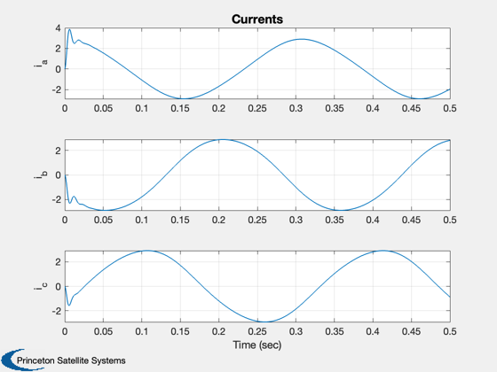
Plot2D( t, xP(1:3,:), tL, {'i_a' 'i_b' 'i_c'}, 'Currents');
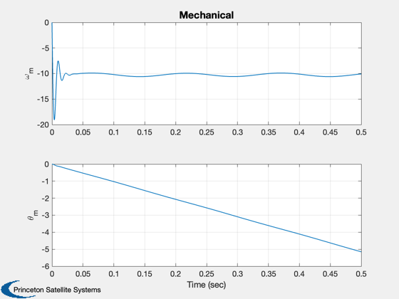
Plot2D( t, xP(4:5,:), tL, {'\omega_m' '\theta_m'}, 'Mechanical');
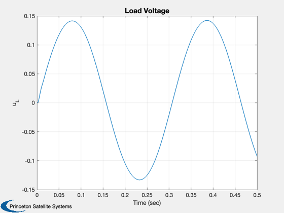
Plot2D( t, xP(6 ,:), tL, {'u_L' }, 'Load Voltage');
%--------------------------------------
% PSS internal file version information
%--------------------------------------
% $Id: 1dc78d9e9e0a605f6ef1b4fdcfd0dd9d8d050ca6 $