Demonstrate LQG control of relative motion in an eccentric orbit

Usage: LQGEccDemo;

------------------------------------------------------------------------

------
Inputs
------
none

-------
Outputs
-------
none

------------------------------------------------------------------------
See also C2DZOH, QHills, QTForm, Mag, RK4TI, LinOrbLQG, FFEccProp,
ECI2Hills, FFEccGoals2Hills, Hills2ECI, Nu2TimeDomain, OrbRate,
AnimationGUI, El2RV, M2Nu, Period, RV2El
------------------------------------------------------------------------

Contents

%-------------------------------------------------------------------------
%   Copyright (c) 2004 Princeton Satellite Systems, Inc.
%   All rights reserved.
%   Since version 7.
%-------------------------------------------------------------------------
%   24-Feb-2017: update output from LinOrbLQG (4 matrices)
%-------------------------------------------------------------------------

%%%%%%%%%%%%%%%%%%%%%%%%%%%%%%%%%%%%%%%%%%%%%%%%%%%%%%%%%%%%%%%%%%%
%%%%%%% BEGIN USER INPUT %%%%%%%%%%%%% BEGIN USER INPUT %%%%%%%%%%%
%%%%%%%%%%%%%%%%%%%%%%%%%%%%%%%%%%%%%%%%%%%%%%%%%%%%%%%%%%%%%%%%%%%

how many orbits to simulate?

nOrbits = 2.0;

after how many orbits do we turn the control on?

tControlOn = 0.05;

orbit parameters

a   = 8000;
e   = 3e-1;
inc = pi/4;

control gains

QG = diag( [5e-3*ones(1,3), 1e-3*ones(1,3)] );  % Scalar estimator gain (make small)
RG = 1e3;                                       % Scalar regulator gain (make big)

noise levels

posSTD = 5.0;  % standard deviation of relative position estimate [cm]
velSTD = 1.0;  % standard deviation of relative position estimate [mm/s]

%%%%%%%%%%%%%%%%%%%%%%%%%%%%%%%%%%%%%%%%%%%%%%%%%%%%%%%%%%%%%%%%%%%
%%%%%%%%%%%%%%%%%%%%%%%%% END USER INPUT %%%%%%%%%%%%%%%%%%%%%%%%%%
%%%%%%%%%%%%%%%%%%%%%%%%%%%%%%%%%%%%%%%%%%%%%%%%%%%%%%%%%%%%%%%%%%%

reference orbit

n     = OrbRate(a);
T     = Period(a);
W     = pi/3;
w     = pi/4;
M     = pi;
el    = [a, inc, W, w, e, M];
[r,v] = El2RV(el);
x0    = [r;v];

simulation time step and duration

dTSim   = 10;

target geometry

gF  = struct('y0',0.0,'xMax',0.25,'nu_xMax',0,'zMax',0,'nu_zMax',0);

compute target trajectory

nu0        = M2Nu(e,el(6));
[xF0,D,dH] = FFEccGoals2Hills( e, nu0, gF, n );

initial relative state

g0  = struct('y0',0.0,'xMax',0.1,'nu_xMax',0,'zMax',0,'nu_zMax',0);
xH0 = FFEccGoals2Hills( e, nu0, g0, n );

second orbit

x1 = Hills2ECI( x0, xH0 );

time vector

t     = 0:dTSim/T:nOrbits;
nSim  = length(t);

generate random noise vector

posSTD = posSTD*1e-5; % standard deviation of relative position error (convert from cm to km)
velSTD = velSTD*1e-6; % standard deviation of relative velocity error (convert from mm/s to km/s)
noise  = [randn(3,nSim)*posSTD; randn(3,nSim)*velSTD];

initialize matrices for plotting

xHEst_plot = zeros(6,nSim);
xHDes_plot = zeros(6,nSim);
xH_plot    = zeros(6,nSim);
aH_plot    = zeros(3,nSim);
nu_plot    = zeros(1,nSim);

aE0 = zeros(3,1);
xK  = xH0;
xH  = xH0;

rhs = @(x,a) [x(4:6); a - (3.98600436e5)*x(1:3)/norm(x(1:3))^3];

for i=1:nSim

   % Hills-frame state estimate
   xHEst = xH + noise(:,i);

   % current desired Hills-frame state
   [el,E,nu] = RV2El( x0(1:3), x0(4:6) );
   xHDes     = FFEccProp( D, nu, el(5), dH );
   xHDes     = Nu2TimeDomain( xHDes, n, el(5), nu );

   if( t(i) > tControlOn )

      % compute new LQG controller
      [AK,BK,CK,DK] = LinOrbLQG( el, QG, RG );
      [AK,BK] = C2DZOH(AK,BK,dTSim);   % discretize with sample time of dTSim

      % update controller
      aH = CK*xK + DK*[xHDes; xHEst];
      xK = AK*xK + BK*[xHDes; xHEst];

   else

      aH = zeros(3,1);

   end

   % rotate Hill's frame acceleration to ECI frame
   qEH = QHills( x0(1:3), x0(4:6) );
   aE1 = QTForm( qEH, aH );

   % integrate
   x0 = RK4TI(rhs,x0,dTSim,aE0);
   x1 = RK4TI(rhs,x1,dTSim,aE1);

   % store for plotting
   aH_plot(:,i)    = aH;
   xH_plot(:,i)    = xH;
   xHDes_plot(:,i) = xHDes;
   xHEst_plot(:,i) = xHEst;
   nu_plot(i)      = nu;

   % Hills-frame state
   xH = ECI2Hills( x0, x1 );

end

assignin('base','t',t);
assignin('base','nu',nu_plot);
assignin('base','xH',xH_plot);
assignin('base','aH',aH_plot);
assignin('base','xHDes',xHDes_plot);
assignin('base','xHEst',xHEst_plot);

k = min( find( tControlOn >= t ) );
fprintf('\n      Total Delta-V: \t %f m/s\n',sum(Mag(aH_plot*dTSim))*1e3)
fprintf(  'Mean Position Error: \t %f m \n\n',mean(Mag(xHDes_plot(1:3,k:end)-xH_plot(1:3,k:end)))*1e3)

      Total Delta-V: 	 2.534435 m/s
Mean Position Error: 	 25.346870 m 

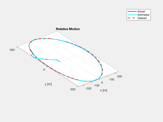
plot trajectory

figure,
plot3(xH_plot(1,:)*1e3,    xH_plot(2,:)*1e3,    xH_plot(3,:)*1e3,          'linewidth',2), hold on
plot3(xHEst_plot(1,:)*1e3, xHEst_plot(2,:)*1e3, xHEst_plot(3,:)*1e3,'c',   'linewidth',2),
plot3(xHDes_plot(1,:)*1e3, xHDes_plot(2,:)*1e3, xHDes_plot(3,:)*1e3,'r--', 'linewidth',2)
title('Relative Motion'), xlabel('x [m]'), ylabel('y [m]'), zlabel('z [m]'), grid on, axis equal, zoom on
legend('Actual','Estimated','Desired');

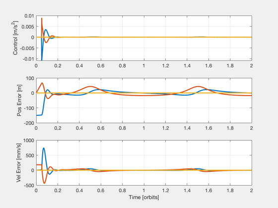
plot control, position error, velocity error

figure,
subplot(311)
plot(t,aH_plot*1e3,'linewidth',2), grid on
ylabel('Control [m/s^2]')
err = xHDes_plot - xHEst_plot;
subplot(312)
plot(t,err(1:3,:)*1e3,'linewidth',2), grid on
ylabel('Pos Error [m]')
subplot(313)
plot(t,err(4:6,:)*1e6,'linewidth',2), grid on
ylabel('Vel Error [mm/s]'), xlabel('Time [orbits]')
zoom on

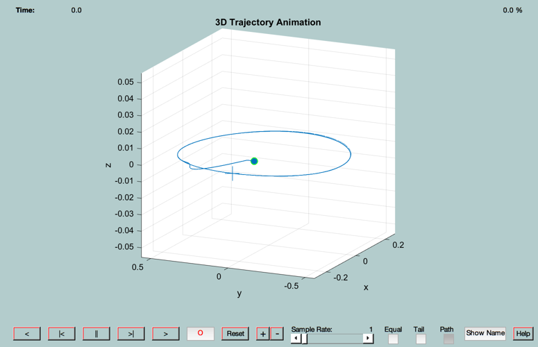
animate

sc    = struct;
sc.r  = xH_plot(1:3,:);
sc.t  = t;
tgt.r = xHDes_plot(1:3,:);
tgt.t = t;
AnimationGUI('initialize',sc,tgt);



%--------------------------------------

Published with MATLAB® R2019a