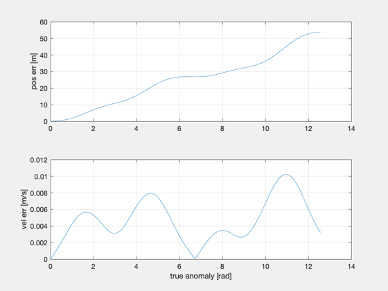
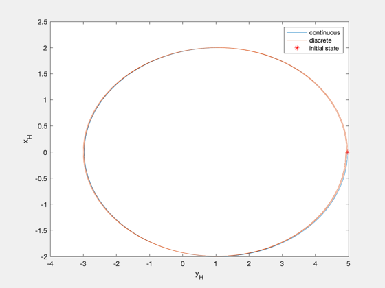
Compare discrete propagation with continuous solution.

This compares FFEccDiscreteHills.m with FFEccLawdensEqns.m

Since version 7.
------------------------------------------------------------------------
Usage:
FFEccPropDemo;
------------------------------------------------------------------------
See also AC, Mag, UnwrapPhase, FFEccDiscreteHills, FFEccLawdensEqns,
FFEccGoals2Hills, Nu2TimeDomain, Time2NuDomain, Nu2M
------------------------------------------------------------------------

%--------------------------------------------------------------------------
%   Copyright (c) 2004 Princeton Satellite Systems, Inc.
%   All rights reserved.
%--------------------------------------------------------------------------

e = 0.03;
n = 1e-3;

nS = 500;

nu0  = 0;
nOrb = 2;
nuF  = nOrb*2*pi;

% evenly spaced true anomaly
nu  = linspace(nu0,nuF,nS+1);
M   = UnwrapPhase(Nu2M(e,nu));
t   = (M-M(1))/n;

% evenly spaced mean anomaly
% M   = linspace(Nu2M(e,nu0),nOrb*2*pi,nS+1);
% nu  = UnwrapPhase(M2Nu(e,M));
% t   = (M-M(1))/n;

g0  = struct('y0',1,'xMax',2,'nu_xMax',pi/2,'zMax',0.5,'nu_zMax',pi);
xH0 = FFEccGoals2Hills( e, nu0, g0, n );

% compute Hills-frame states using discrete propagation
aC     = zeros(3,nS);
xHDisc = FFEccDiscreteHills( e, n, xH0, nu0, aC, t );

% compute Hills-frame states using solution to continuous equations
xH0nu  = Time2NuDomain( xH0, n, e, nu0 );
xHCont = FFEccLawdensEqns( xH0nu, nu0, nu, e );
xHCont = Nu2TimeDomain( xHCont, n, e, nu );

% error
xE = (xHCont - xHDisc)*1e3;

figure
subplot(211)
plot(nu,Mag(xE(1:3,:))), grid on, ylabel('pos err [m]')
subplot(212)
plot(nu,Mag(xE(4:6,:))), grid on, ylabel('vel err [m/s]'), xlabel('true anomaly [rad]')

figure,
plot(xHCont(2,:),xHCont(1,:),xHDisc(2,:),xHDisc(1,:)), hold on
plot(xHDisc(2,1),xHDisc(1,1),'r*'), xlabel('y_H'), ylabel('x_H')
legend('continuous','discrete','initial state')

%--------------------------------------

Published with MATLAB® R2020a