Contents

Demonstrate rendezvous control with PD or LQ

This allows for both a PD controller and LQ (linear quadratic) controller. Both work in continuous time. Script contains an embedded RHS function.

See also LinOrb, QCR, Riccati, DispWithTitle, TimeLabl, RK4, Odd

%--------------------------------------------------------------------------
%   Copyright (c) 2020 Princeton Satellite Systems, Inc.
%   All rights reserved.
%--------------------------------------------------------------------------

Constants

m     = 1000;
dT    = 1;
d.n   = 2*pi/(90*60);
useLQ = true;

Design a quadratic regulator

[a, b]  = LinOrb( [], d.n );
kLQ     = QCR( a, b, eye(6), 1e5*eye(3) );

DispWithTitle(kLQ,'Gain Matrix LQ')
DispWithTitle(eig(a-b*kLQ),'LQ eigenvalues')

Gain Matrix LQ
     0.003165  -9.2471e-05  -3.2574e-19     0.079624    7.462e-07  -1.4935e-18
   9.2471e-05    0.0031609  -5.3816e-19    7.462e-07     0.079573   -1.041e-17
   1.1592e-20   -3.251e-19    0.0031609   1.9551e-19  -3.3105e-18     0.079573
LQ eigenvalues
    -0.039801 +   0.040891i
    -0.039801 -   0.040891i
    -0.039798 +   0.038564i
    -0.039798 -   0.038564i
    -0.039786 +   0.039741i
    -0.039786 -   0.039741i

Design a PD controller

zeta  = 1;
omega = 0.06; % Omega must be faster than n
kPD   = [omega^2*eye(3) 2*zeta*omega*eye(3)];

DispWithTitle(kPD,'Gain Matrix PD')
DispWithTitle(eig(a-b*kLQ),'PD eigenvalues')

Gain Matrix PD
       0.0036            0            0         0.12            0            0
            0       0.0036            0            0         0.12            0
            0            0       0.0036            0            0         0.12
PD eigenvalues
    -0.039801 +   0.040891i
    -0.039801 -   0.040891i
    -0.039798 +   0.038564i
    -0.039798 -   0.038564i
    -0.039786 +   0.039741i
    -0.039786 -   0.039741i

Simulation

x     = [1;1;1;0.01;0.01;0.01];
xP    = zeros(9,m);
for k = 1:m
  if( useLQ)
    d.aD    = -kLQ*x; %#ok<*UNRCH>
  else
    d.aD    = -kPD*x;
  end
  xP(:,k) = [x;d.aD];
  x       = RK4( @RHS, x, dT, 0, d );
end

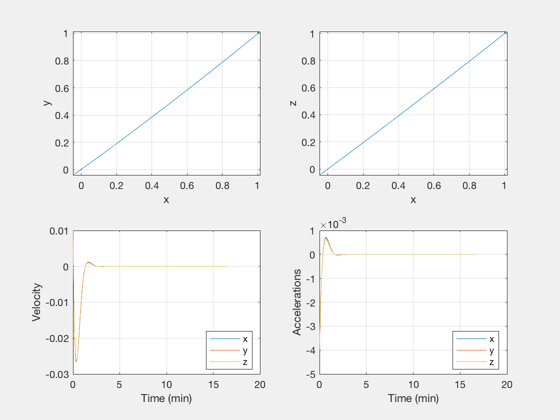
Plotting

t = (0:m-1)*dT;
h = figure;
if( useLQ )
  s = 'Rendezvous LQ Controller';
else
  s = 'Rendezvous PD Controller';
end

set(h,'name',s)
subplot(2,2,1)
plot(xP(1,:),xP(2,:))
grid on
xlabel('x');
ylabel('y')

subplot(2,2,2)
plot(xP(1,:),xP(3,:))
grid on
xlabel('x');
ylabel('z')

[t,tL] = TimeLabl(t);
subplot(2,2,3)
plot(t,xP(4:6,:))
grid on
xlabel(tL);
ylabel('Velocity')
legend('x','y','z','location','best')

subplot(2,2,4)
plot(t,xP(7:9,:))
grid on
xlabel(tL);
ylabel('Accelerations')
legend('x','y','z','location','best')

Hills equations

function xDot = RHS(x,~,d)

nSq   = d.n^2;
xDot  = [x(4:6);d.aD+[2*d.n*x(5)+3*nSq*x(1);-2*d.n*x(4);-nSq*x(3)]];

end



%--------------------------------------

Published with MATLAB® R2019a