Apophis 3D optimal trajectory with a linear regulator

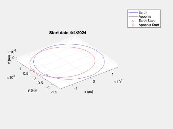
Starts with plotting the Earth and Apophis orbits. It then uses an optimal regulator to do the transfer with a linearized orbit.

------------------------------------------------------------------------
See also Constant, ApophisOrbit, AdjustMeanAnomaly, RVOrbGen,
PlanetPosJPL, NewFig, JD2Date, ECI2Hills, OrbRate, RHSLinOrb,
QCR, RK4, TimeHistory
------------------------------------------------------------------------

Contents

%--------------------------------------------------------------------------
%   Copyright (c) 2023.1 Princeton Satellite Systems, Inc.
%   All rights reserved.
%--------------------------------------------------------------------------
%   Since 2023.1
%--------------------------------------------------------------------------

Constants

dayToSec      = 86400;
mu            = Constant('mu sun');

Generate the Earth and Apophis orbit

[elA,~,~,jDA] = ApophisOrbit;
jD0           = Date2JD([2024 4 4]);
el            = AdjustMeanAnomaly(elA,jDA,jD0);
nDays         = 500;
t             = 0:nDays;
jD            = jD0 + t;
[rApophis,vApophis] = RVOrbGen(elA,t*dayToSec,[],mu);

PlanetPosJPL( 'initialize', 3 );

rEarth = zeros(3,length(jD));
vEarth = zeros(3,length(jD));

for k = 1:length(jD)
  [rEarth(:,k),~,vEarth(:,k)] = PlanetPosJPL( 'update', jD(k), 1 );
end

NewFig('Apophis and Earth')
plot3(rEarth(1,:),rEarth(2,:),rEarth(3,:),'b');
hold on
plot3(rApophis(1,:),rApophis(2,:),rApophis(3,:),'r');
XLabelS('x (au)');
YLabelS('y (au)');
ZLabelS('z (au)');
axis image
grid on
rotate3d on
plot3(rEarth(1,1),rEarth(2,1),rEarth(3,1),'ob');
hold on
dS = JD2Date(jD0);
title(sprintf('Start date %d/%d/%d',dS(2),dS(3),dS(1)));
plot3(rApophis(1,1),rApophis(2,1),rApophis(3,1),'or');

hold off
legend('Earth','Apophis','Earth Start', 'Apophis Start')

Use a linear quadratic regulator with a linearized orbit to simulation the trajectory

% Find Hills Coordinates for Apophis
xA = RelativeOrbitState([rEarth(:,1);vEarth(:,1)],[rApophis(:,1);vApophis(:,1)]);
n  = OrbRate(Mag(rEarth(:,1)),Mag(rEarth(:,1)),mu);

x    = zeros(6,1);
dT   = 100; % sec
nYrs = 0.8;
tEnd = nYrs*365.25*dayToSec;
nSim = floor(tEnd/dT);
xP   = zeros(13,nSim);
u    = zeros(3,1);

% Find the optimal gains
[~,a,b] = RHSLinOrb(zeros(6,1),0,n,u);

% Create the linear quadratic regulator. Pick a large value for the control
% weight
kOpt = QCR(a,b,eye(6),eye(3)*1e26)

% Check the eigenvalues
DispWithTitle(eig(a-b*kOpt),'Controller Eigenvalues')

% Simulate
TimeDisplay( 'initialize', 'Apophis Optimal Trajectory', nSim );
for k = 1:nSim
  xP(:,k) = [xA;x;Mag(u)];
  xA      = RK4(@RHSLinOrb,xA,dT,0,n,zeros(3,1));
  u       = kOpt*(xA-x);
  x       = RK4(@RHSLinOrb,x,dT,0,n,u);
  TimeDisplay( 'update' );
end
TimeDisplay( 'close' );

kOpt =

   2.0682e-13   -8.243e-14   2.8263e-29   5.6796e-07   1.0144e-07    3.424e-22
   1.2805e-13   5.6615e-14  -9.9089e-29   1.0144e-07   4.2862e-07  -1.7579e-22
  -3.6116e-30   3.5087e-30   6.7939e-14  -1.5511e-23   6.5709e-25   3.6862e-07

Controller Eigenvalues
  -2.3214e-07 + 4.0477e-07i
  -2.3214e-07 - 4.0477e-07i
  -2.6615e-07 + 2.2681e-08i
  -2.6615e-07 - 2.2681e-08i
  -1.8431e-07 + 2.7128e-07i
  -1.8431e-07 - 2.7128e-07i

Plot

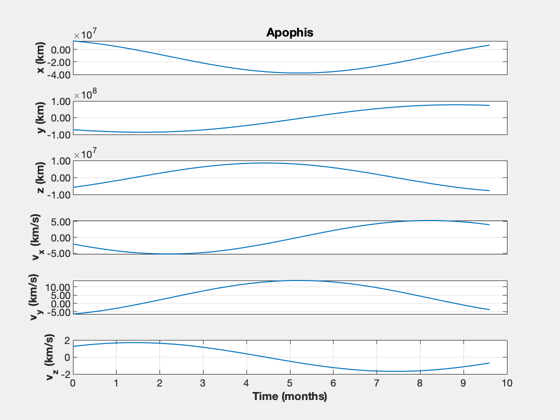
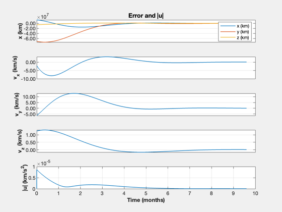
The required control acceleration is the magnitude of u, u

yL = {'x (km)' 'y (km)' 'z (km)' 'v_x (km/s)' 'v_y (km/s)' 'v_z (km/s)'...
      '|u| (km/s^2)'};

t = (0:nSim-1)*dT;
k = 1:6;
TimeHistory(t,xP(k,:),yL(1:6),'Apophis');
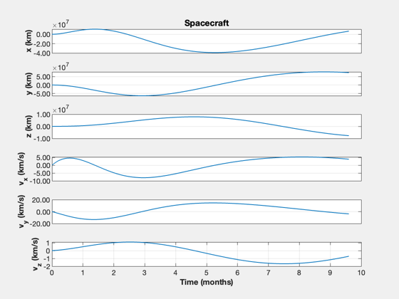
k = 7:12;
TimeHistory(t,xP(k,:),yL(1:6),'Spacecraft');
e = xP(1:6,:) - xP(7:12,:);
TimeHistory(t,[e;xP(13,:)],yL([1 4:7]),'Error and |u|',{[1 2 3],4,5,6,7},...
  {yL(1:3),{},{},{},{}});

fprintf('Delta-V: %g km/s\n',trapz(xP(13,:))*dT)

%--------------------------------------

% $Id: ff06d4f17f188f9d49ba0d76ddcca6d16c66a30c $

Delta-V: 26.5531 km/s

Published with MATLAB® R2024a