Mars 3D optimal trajectory with a linear regulator

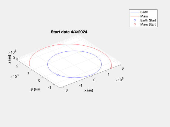
Starts with plotting the Earth and Mars orbits. It then uses an optimal regulator to do the transfer with a linearized orbit. This nulls the error but has no limits on acceleration so requires a high delta-V.

------------------------------------------------------------------------
See also Constant, PlanetPosJPL, NewFig, JD2Date, ECI2Hills,
OrbRate, RHSLinOrb, QCR, RK4, TimeHistory
------------------------------------------------------------------------

Constants
Initialize the planetary ephemerides
Time
Use a linear quadratic regulator with a linearized orbit to simulate the trajectory
Nonlinear simulation

%--------------------------------------------------------------------------
%   Copyright (c) 2023.1 Princeton Satellite Systems, Inc.
%   All rights reserved.
%--------------------------------------------------------------------------
%   Since 2023.1
%--------------------------------------------------------------------------

Constants

dayToSec = 86400;
MU       = Constant('mu sun');

Initialize the planetary ephemerides

PlanetPosJPL( 'initialize', [3 4] );

Time

jD0   = Date2JD([2024 4 4]);
nYr   = 1;
nDays = nYr*365.25;
t     = 0:nDays;
jD    = jD0 + t;

nS     = length(jD);
rMars  = zeros(3,nS);
rEarth = zeros(3,nS);
vMars  = zeros(3,nS);
vEarth = zeros(3,nS);

for k = 1:nS
  [r,~,v]     = PlanetPosJPL( 'update', jD(k), 1 );
  rEarth(:,k) = r(:,1);
  vEarth(:,k) = v(:,1);
  rMars(:,k)  = r(:,2);
  vMars(:,k)  = v(:,2);
end

NewFig('Mars and Earth')
plot3(rEarth(1,:),rEarth(2,:),rEarth(3,:),'b');
hold on
plot3(rMars(1,:),rMars(2,:),rMars(3,:),'r');
XLabelS('x (au)');
YLabelS('y (au)');
ZLabelS('z (au)');
axis image
grid on
rotate3d on
plot3(rEarth(1,1),rEarth(2,1),rEarth(3,1),'ob');
hold on
dS = JD2Date(jD0);
title(sprintf('Start date %d/%d/%d',dS(2),dS(3),dS(1)));
plot3(rMars(1,1),rMars(2,1),rMars(3,1),'or');

hold off
legend('Earth','Mars','Earth Start', 'Mars Start')

Use a linear quadratic regulator with a linearized orbit to simulate the trajectory

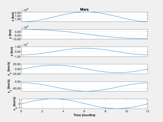
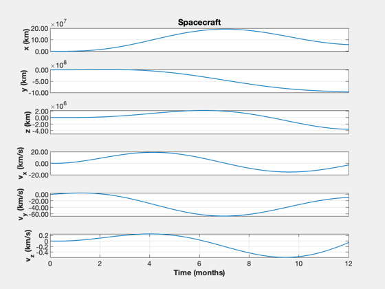
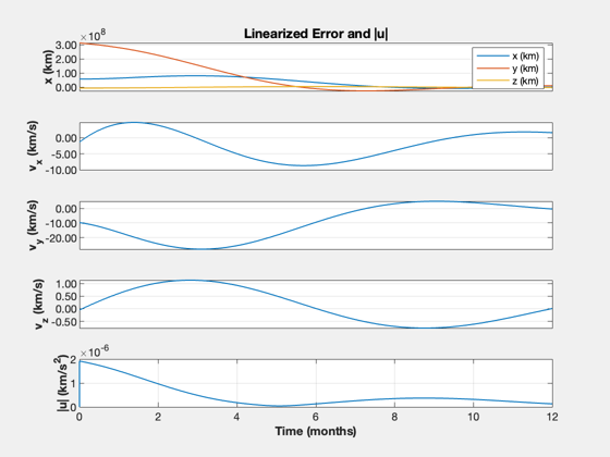
% Find Hills Coordinates for Mars
xM = RelativeOrbitState([rEarth(:,1);vEarth(:,1)],[rMars(:,1);vMars(:,1)]);
n  = OrbRate(Mag(rEarth(:,1)),Mag(rEarth(:,1)),MU);
% Todo: confirm we can recreate the inertial orbit of Mars, or at least
% compare

x    = zeros(6,1);
dT   = 200; % s
tEnd = nYr*365.25*dayToSec;
nSim = floor(tEnd/dT);
xP   = zeros(13,nSim);
u    = zeros(3,1);

% Linearize around the Earth's orbit; assumes small x, z
[~,a,b] = RHSLinOrb(zeros(6,1),0,n,u);

% Find the optimal gains
% Create the linear quadratic regulator. Pick a large value for the control
% weight
gain = 1e28;
kOpt = QCR(a,b,eye(6),eye(3)*gain)

% Check the eigenvalues
DispWithTitle(eig(a-b*kOpt),'Controller Eigenvalues')

% Linearized continous orbit RHS
funRHS = @(x,t,u) a*x + b*u ;

% Simulate
TimeDisplay( 'initialize', 'Mars Optimal Trajectory', nSim );
t = 0;
for k = 1:nSim
  xP(:,k) = [xM;x;Mag(u)];
  xM      = RK4(funRHS,xM,dT,0,zeros(3,1));
  u       = kOpt*(xM-x);
  x       = RK4(funRHS,x,dT,0,u);
  TimeDisplay( 'update' );
end
TimeDisplay( 'close' );

% Plot the linear solution
% The required control acceleration is the magnitude of u, |u|

fprintf('Delta-V, linearized: %g km/s\n',trapz(xP(13,:))*dT)

yL = {'x (km)' 'y (km)' 'z (km)' 'v_x (km/s)' 'v_y (km/s)' 'v_z (km/s)'...
      '|u| (km/s^2)'};

t = (0:nSim-1)*dT;
k = 1:6;
TimeHistory(t,xP(k,:),yL(1:6),'Mars');
k = 7:12;
TimeHistory(t,xP(k,:),yL(1:6),'Spacecraft');
e = xP(1:6,:) - xP(7:12,:);
TimeHistory(t,[e;xP(13,:)],yL([1 4:7]),'Linearized Error and |u|',{[1 2 3],4,5,6,7},...
  {yL(1:3),{},{},{},{}});

kOpt =

    6.107e-14  -8.7476e-15  -5.7204e-29   1.3463e-07   1.1424e-07  -3.9822e-22
   1.0435e-13  -4.8455e-15   3.6456e-29   1.1424e-07   2.6119e-07   -1.098e-21
  -1.7608e-29   4.7334e-30   1.2423e-15  -1.7577e-22  -1.9347e-23   4.9847e-08

Controller Eigenvalues
  -7.3109e-08 + 2.3871e-07i
  -7.3109e-08 - 2.3871e-07i
   -1.248e-07 + 5.9708e-08i
   -1.248e-07 - 5.9708e-08i
  -2.4923e-08 + 2.0061e-07i
  -2.4923e-08 - 2.0061e-07i

Delta-V, linearized: 15.2919 km/s

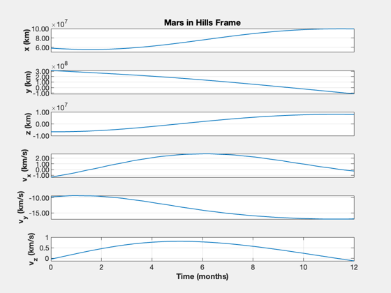
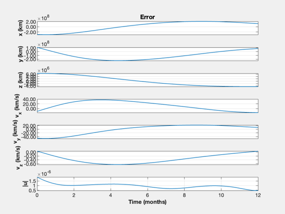
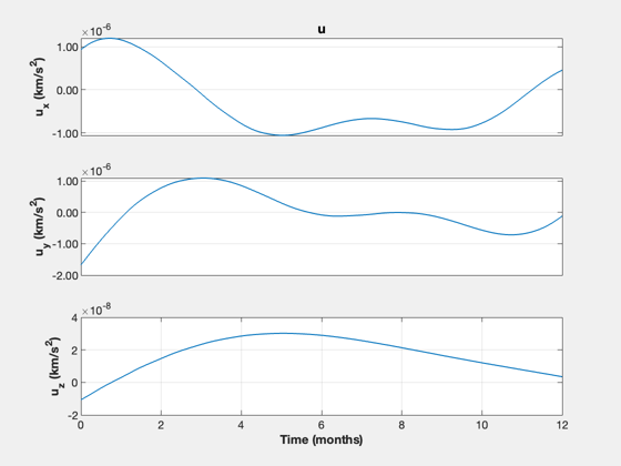
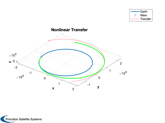
Nonlinear simulation

See how the linear controller performs with nonlinear dynamics.

% Time
nSim = floor(tEnd/dT);
t  = (0:nSim-1)*dT;
jD = jD0 + t/86400;

% Initialization
x0    = [rEarth(:,1);vEarth(:,1)];
rE    = zeros(3,nSim);
vE    = zeros(3,nSim);
rMars = zeros(3,nSim);
vMars = zeros(3,nSim);
xP    = zeros(15,nSim);

% Simulate
x    = x0(:,1);
TimeDisplay( 'initialize', 'Mars Nonlinear Optimal Trajectory', nSim );
for k = 1:nSim
  % Obtain planet states
  [r,~,v]     = PlanetPosJPL( 'update', jD(k), 1 );
  rE(:,k)     = r(:,1);
  vE(:,k)     = v(:,1);
  rMars(:,k)  = r(:,2);
  vMars(:,k)  = v(:,2);
  x0 = [rE(:,k);vE(:,k)];
  % Get the relative state
  xM      = RelativeOrbitState(x0,[rMars(:,k);vMars(:,k)]);
  xH      = RelativeOrbitState(x0,x);
  % Calculate the linear control and rotate it
  cH      = GetHillsMats( rE(:,k), vE(:,k) );
  uH      = cH'*kOpt*(xM - xH);
  xP(:,k) = [x;xM;uH];
  % Integrate the nonlinear orbit
  x       = RK4(@FOrbCart,x,dT,0,uH,MU);
  TimeDisplay( 'update' );
end
TimeDisplay( 'close' );

yL = {'x (km)' 'y (km)' 'z (km)' 'v_x (km/s)' 'v_y (km/s)' 'v_z (km/s)', '|u|'};

TimeHistory(t,xP(7:12,:),yL(1:6),'Mars in Hills Frame');

e = xP(1:6,:) - [rMars;vMars];
u = Mag(xP(13:15,:));
TimeHistory(t,[e;u],yL,'Error');
yL = {'u_x (km/s^2)' 'u_y (km/s^2)' 'u_z (km/s^2)'};

TimeHistory(t,xP(13:15,:),yL,'u');

fprintf('Delta-V, nonlinear: %g km/s\n',trapz(u)*dT)

Plot3D(rEarth,'x','y','z','Nonlinear Transfer');
hold on
plot3(rEarth(1,1),rEarth(2,1),rEarth(3,1),'bo');
plot3(rMars(1,:),rMars(2,:),rMars(3,:),'r');
plot3(rMars(1,end),rMars(2,end),rMars(3,end),'rx');
plot3(xP(1,:),xP(2,:),xP(3,:),'g','linewidth',2);
legend('Earth','Mars','Transfer')


%--------------------------------------

% $Id: 45f2292f0443b52c613978433b5d21a12b280b44 $