Contents
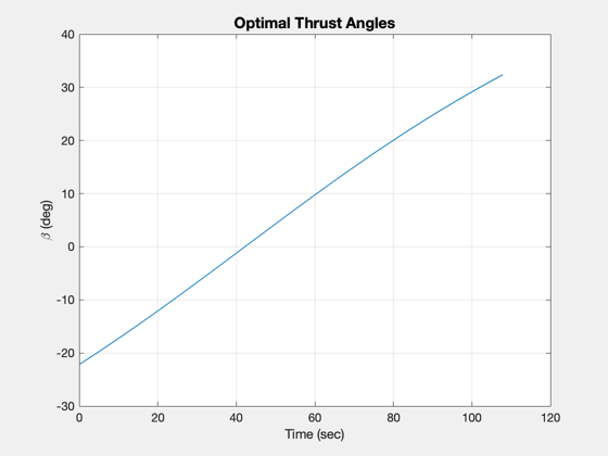
3D lander simulation using the bilinear tangent law.
The spacecraft has 3-axis thruster control. Ideal attitude pointing is assumed. An altimeter gives the altitude. The planet is assumed to be a perfect sphere. The dynamics model accounts for the changing mass of the vehicle as fuel is consumed.
This demo demonstrates the bilinear tangent law for descent from a circular equatorial orbit. Choose between the moon, Mars, and Enceladus, or add your own body.
Things to explore:
1. For the bilinear control, vary the control acceleration (nAccel).
2. Try different starting altitudes.
3. Try different planets: moon, Mars, Enceladus
%--------------------------------------------------------------------------
% See also: LandingControlBilinear, Inertias, RHSPointMass, RK4, Plot2D
%--------------------------------------------------------------------------
%--------------------------------------------------------------------------
%   Copyright (c) 2013-2014 Princeton Satellite Systems, Inc.
%   All rights reserved.
%--------------------------------------------------------------------------
%   Since version 2014.1
%--------------------------------------------------------------------------
Simulation time parameters
%--------------------------------------
dT              = 0.25; % sec
Parameters
%------------
hStop           = 0.0005; % km
uE              = 320*9.806; % Exhaust velocity (m/s)

% Select the planet or moon
%--------------------------
body            =  'moon'; %'Moon'; %'Mars';'enceladus'

% Planet/moon parameters
%-----------------------
d = struct;
switch lower(body)
  case 'moon'
    rPlanet             = Constant('equatorial radius moon'); % km
    muPlanet            = Constant('mu moon');
    h                   = 15;  % Altitude of initial orbit
    tEnd                = 7*60; % sec
    nAccel              = 10; % Engine acceleration is this multiple of gravity
    massFuel            = 25;
    d.mass              = 25; % kg
    gainVelocity        = 2;
    velocityThreshold   = 0.001;
    vMaxFrac            = 0.2;

  case 'enceladus'
    rPlanet             = 252.1; % km
    muPlanet            = 1.08022e20*Constant('newtonian constant of gravitation')/1e9;
    h                   = 10;  % Altitude of initial orbit
    tEnd                = 10*60; % sec
    nAccel              = 8; % Engine acceleration is this multiple of gravity
    massFuel            = 8;
    d.mass              = 100; % kg
    gainVelocity        = 0.5;
    velocityThreshold   = 0.001;
    vMaxFrac            = 0.2;

  case 'mars'
    rPlanet             = Constant('equatorial radius mars'); % km
    muPlanet            = Constant('mu mars');
    h                   = 150; % Altitude of initial orbit
    nAccel              = 7; % Engine acceleration is this multiple of gravity
    tEnd                = 5*60; % sec
    massFuel            = 1000;
    d.mass              = 200; % kg
    gainVelocity        = 4;
    velocityThreshold   = 0.001;
    vMaxFrac            = 0.2;

end

% Simulation time steps
%----------------------
nSim            = floor(tEnd/dT);

% Spacecraft inertia at start
%----------------------------
d.inertia       = Inertias( d.mass + massFuel, [1 1 1], 'box', 1 ); % kg-m^2
Set up the bilinear controller
%--------------------------------
dBilinear = struct;
dBilinear.mu                        = muPlanet;
dBilinear.mass                      = d.mass + massFuel;
dBilinear.rP                        = rPlanet;
dBilinear.h                         = h;
dBilinear.nG                        = nAccel;
dBilinear.dT                        = dT;
dBilinear.inertia                   = d.inertia;
dBilinear.hLanding                  = 0.1; % The altitude at which to switch to landing mode
dBilinear.throttle                  = 1;
dBilinear.landing.gainVelocity      = gainVelocity;
dBilinear.landing.velocityThreshold = velocityThreshold;
dBilinear.landing.vMaxFrac          = vMaxFrac;
dBilinear.landing.hTouchdown        = 0.001;
dBilinear.bypassACS                 = 1;
dBilinear                           = LandingControlBilinear( 'initialize', dBilinear );

% Determine initial s/c orientation (align s/c with initial beta angle)
%------------------------------------------------------------------
d.hLanding                          = dBilinear.hLanding;
Descent duration 107.8732 sec
Simulation
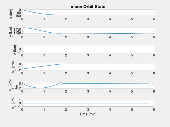
%------------

% Gravity
%--------
d.mu    = muPlanet; % km^3/s^2

% Disturbances
%-------------
d.fDist = []; % The landing force function

% State vector [r;v;mass fuel]
% Assume a circular orbit to start
%---------------------------------
r = rPlanet + h;
u = sqrt(muPlanet/r);
x = [0;r;0;-u;0;0;massFuel];

% Initialize state vector array for plotting
%-------------------------------------------
xP = zeros(length(x)+3,nSim);

% Initialize time
%----------------
t = 0;

% Simulate until the lander reaches the surface (within 1 mm)
%------------------------------------------------------------
for k = 1:nSim

  % Sensing - determine altitude
  %-----------------------------
  hAltimeter = Mag(x(1:3)) - rPlanet;
  massFuel   = x(7);

  % Controller
  %-----------
  dBilinear.mass       	= d.mass + massFuel;
  dBilinear.r         	= x(1:3);
  dBilinear.v          	= x(4:6);
  dBilinear.hAltimeter	= hAltimeter;
  dBilinear.t          	= t;
  dBilinear.pointingTol = 0.001;
  dBilinear            	= LandingControlBilinear('update',dBilinear);
  d.forceECI           	= dBilinear.forceECI;

  % Store for plotting
  %-------------------
  xP(:,k) = [x;hAltimeter;dBilinear.throttle;dBilinear.mode];

  % Stop when we reach the surface or run out of fuel
  %--------------------------------------------------
  if( dBilinear.landing.mode == 4 )
    fprintf(1,'Touchdown! |v| = %12.4f km/s\n',Mag(x(4:6)));
    break
  end

  if( hAltimeter <= hStop )
    fprintf(1,'Terminating due to hitting the ground. |v| = %12.4f km/s\n',Mag(x(4:6)));
    break
  end

  if( massFuel  <= 0 )
    fprintf(1,'Terminating due to running out of fuel. |v| = %12.4f km/s h = %12.4 km\n',Mag(x(4:6)),hAltimeter);
    break
  end

  % Fuel consumption
  %-----------------
  d.mDot = -abs(Mag(d.forceECI))/uE;

  % Integrate
  %----------
  x = RK4(@RHSPointMass,x,dT,t,d);

  % Increment time
  %---------------
  t = t + dT;
end
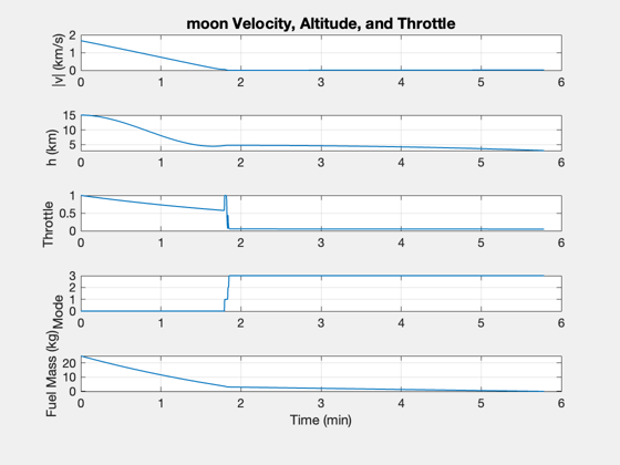
Altitude       4.7780
Free-fall velocity       0.0878
Maximum allowed velocity       0.0176
Terminating due to running out of fuel. |v| =       0.0151 km/s h =
Plot the simulation results
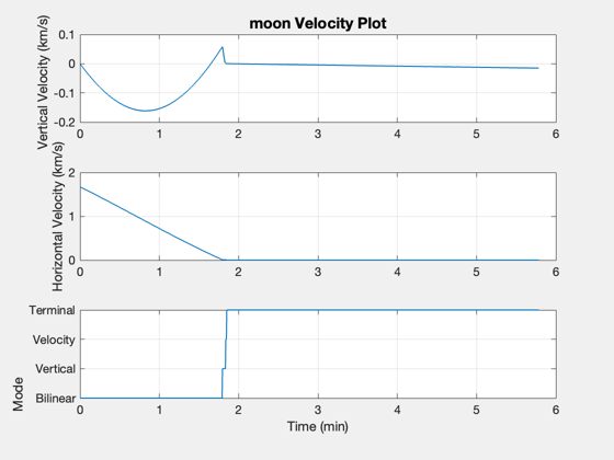
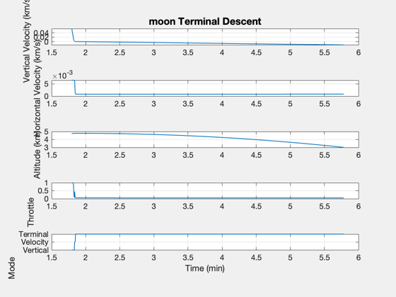
%-----------------------------
xP = xP(:,1:k);

% Time label
%-----------
[t,tL] = TimeLabl((0:(k-1))*dT);

% Plot Titles
%------------
s1 = sprintf('%s Orbit State',body);
s2 = sprintf('%s Velocity, Altitude, and Throttle',body);
s3 = sprintf('%s Terminal Descent',body);

% Plot position in ECI frame
%---------------------------
yL = {'x (km)','y (km)','z (km)','v_x (km)','v_y (km)','v_z (km)'};
Plot2D( t, xP(  1:6,:), tL, yL, s1 )

% Summary plot
%-------------
yL = {'|v| (km/s)' ,'h (km)', 'Throttle' 'Mode' , 'Fuel Mass (kg)'};
Plot2D( t, [Mag(xP(4:6,:));xP([8 9 10 7],:)], tL, yL, s2);

% Velocity plot
%--------------
uV = Unit(xP(1:3,:));
vV = Dot(uV,xP(4:6,:));
vH = Mag(xP(4:6,:) - uV.*[vV;vV;vV]);
s2 = sprintf('%s Velocity Plot',body);
Plot2D( t, [vV;vH;xP(10,:)], tL, {'Vertical Velocity (km/s)' 'Horizontal Velocity (km/s)' 'Mode'},s2)
subplot(3,1,3)
set(gca,'YTick',[0 1 2 3 4],'YTickMode','manual',...
  'YTickLabel',{'Bilinear' 'Vertical' 'Velocity' 'Terminal' 'Touchdown'})

% Generate a terminal maneuvering plot
%-------------------------------------
kT = find(xP(10,:) > 0 );
vV = vV(kT);
vH = vH(kT);
xP = xP(8:10,kT);
t  = t(kT);

Plot2D( t, [vV;vH;xP], tL, {'Vertical Velocity (km/s)' 'Horizontal Velocity (km/s)' 'Altitude (km)' 'Throttle' 'Mode'},s3)
subplot(5,1,5)
set(gca,'YTick',[0 1 2 3 4],'YTickMode','manual',...
  'YTickLabel',{'Bilinear' 'Vertical' 'Velocity' 'Terminal' 'Touchdown'})

%--------------------------------------

% $Id: 5d3f118ba3c37ae4ab8336a019e01eeffe1d408a $