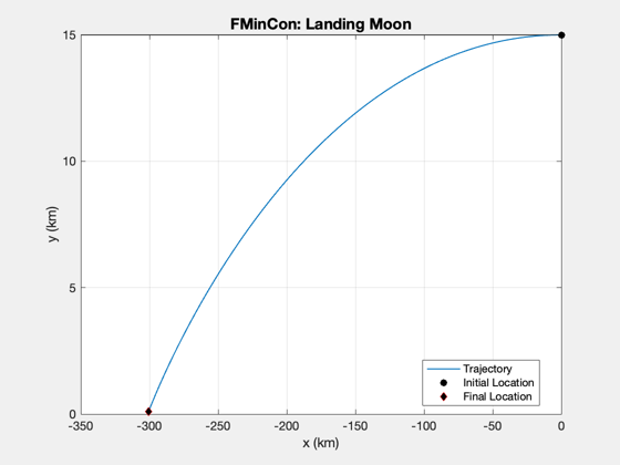
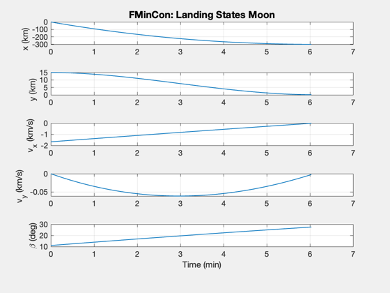
Compute a minimum time landing trajectory using fmincon
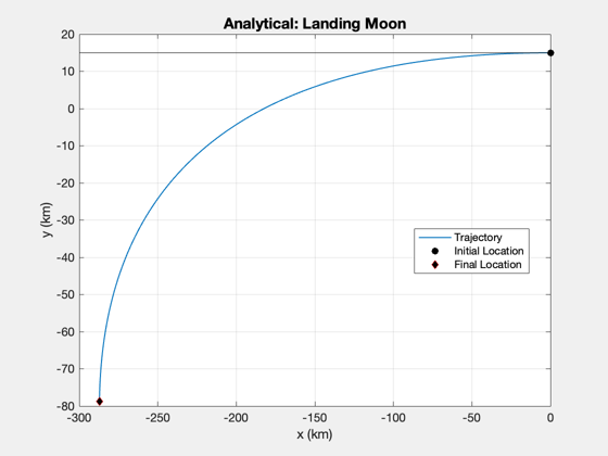
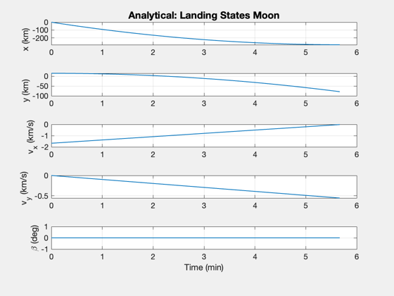
The test is for a lunar landing in 2D. The surface is assumed flat. The acceleration is constant. Start from zero angles.
Requires fmincon from the MATLAB Optimization Toolbox.
See also: Constant, Simulate2DLanding, LandingCost2D, LandingConst2D
Contents
%--------------------------------------------------------------------------
%   Copyright (c) 2021 Princeton Satellite Systems, Inc.
%   All rights reserved.
%--------------------------------------------------------------------------
%   Since version 2021.1
%--------------------------------------------------------------------------

if( ~HasOptimizationToolbox )
  error('You need the MATLAB optimizaton toolbox to run this script.');
end
Parameters
muMoon      = Constant('mu moon');
rMoon       = Constant('equatorial radius moon');
d           = struct;
d.n         = 100; % Number of increments
d.g         = muMoon/rMoon^2; % Gravity
d.a         = 3*d.g; % Engine acceleration
h           = 15; % km

% Thrust direction angles, start with zero
beta        = zeros(1,d.n);

% The initial state is [0;h;-u;0]
r           = rMoon + h;
x           = [0;h;-sqrt(muMoon/r);0];
tMin        = abs(x(3))/d.a;
t           = linspace(0,tMin,d.n+1);
d.x         = x;
d.hFinal    = 0.1;

% Simulate the landing
Simulate2DLanding( t, beta, d, 'Analytical' );
Now repeat with fmincon
% fmincon options
opts      = optimset('Display','iter-detailed',...
                     'TolFun',1e-4,...
                     'algorithm','interior-point',...
                     'TolCon',1e-5,...
                     'MaxFunEvals',10000);

% Pass the initial state to the optimizer
d.x =  x;

% The cost is time, which is a decision variable
% The cost is the time to reach the final state vector
costFun   = @(x) LandingCost2D(x,d);

% The numerical integration of the state is in the constraint function
constFun	= @(x) LandingConst2D(x,d);

% The final state vector is [x;0;0;0];
% We don't care what x is since we can always start the descent at the
% appropriate time.

% First guess for the time decision variable
dT        = t(2:end) - t(1:end-1);

% The decision variables are acceleration angle and time increment
u0        = [beta';dT'];

% Lower and upper bounds
lB        = [-(pi/2)*ones(length(dT),1);zeros(length(dT),1)];
uB        = [(pi/2)*ones(length(dT),1);100*ones(length(dT),1)];

% Find the optimal decision variables.
u         = fmincon(costFun,u0,[],[],[],[],lB,uB,constFun,opts);
                                            First-order      Norm of
 Iter F-count            f(x)  Feasibility   optimality         step
    0     201    3.434516e+02    8.083e+01    2.301e-06
    1     402    3.434516e+02    1.288e+00    1.171e+00    3.452e+00
    2     603    3.656850e+02    3.730e-01    2.252e-01    2.229e+00
    3     804    3.656580e+02    2.840e-02    2.023e-01    2.740e-01
    4    1005    3.656738e+02    1.243e-02    9.136e-02    1.846e-01
    5    1206    3.657437e+02    1.729e-04    1.888e-02    2.281e-02
    6    1407    3.657436e+02    1.012e-04    3.439e-04    1.587e-02
    7    1608    3.657441e+02    9.527e-07    1.455e-03    1.514e-03
    8    1809    3.657441e+02    5.146e-07    1.834e-04    1.142e-03
    9    2010    3.657441e+02    6.149e-09    1.264e-04    1.246e-04
   10    2211    3.657441e+02    3.513e-09    3.668e-05    9.394e-05

Optimization completed: The relative first-order optimality measure, 3.668402e-05,
is less than options.OptimalityTolerance = 1.000000e-04, and the relative maximum constraint
violation, 4.345736e-11, is less than options.ConstraintTolerance = 1.000000e-05.
Set up the simulation
beta      = u(1:d.n)';
dT        = u(d.n+1:2*d.n);
t         = zeros(1,length(dT));
for k = 2:d.n+1
  t(k) = t(k-1) + dT(k-1);
end

% Simulate the landing
Simulate2DLanding( t, beta, d, 'FMinCon' );


%--------------------------------------

% $Id: 39517411025e420dc8378b74d7c4215f0d64649d $