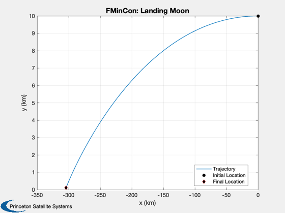
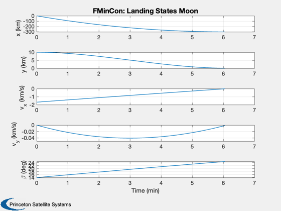
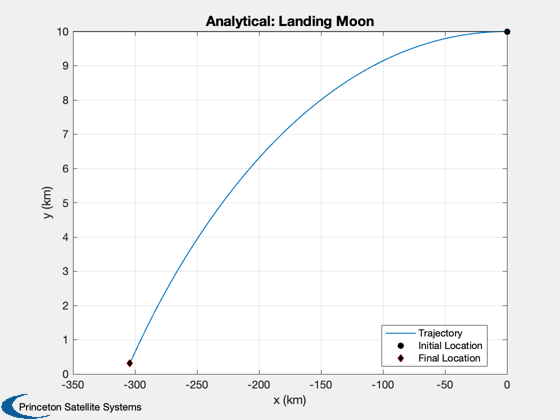
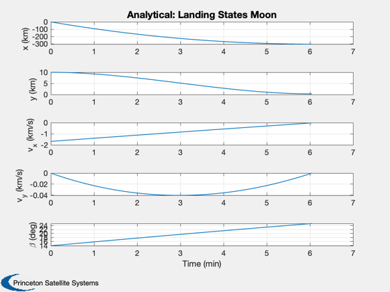
Test fmincon against an analytical solution for the linear tangent law
The test is for a lunar landing in 2D. The surface is assumed flat. The acceleration is constant. Assumes u is along -x.
Requires fmincon from the MATLAB Optimization Toolbox.
See also: Constant, BilinearTangentLaw, Simulate2DLanding, LandingCost2D, LandingConst2D
Contents
%--------------------------------------------------------------------------
%   Copyright (c) 2015 Princeton Satellite Systems, Inc.
%   All rights reserved.
%--------------------------------------------------------------------------
%   Since 2016.1
%--------------------------------------------------------------------------

if( ~HasOptimizationToolbox )
  error('You need the MATLAB optimizaton toolbox to run this script.');
end

MU_MOON = Constant('mu moon');
R_MOON  = Constant('equatorial radius moon');
Parameters
% Initial state
h  = 10; % Altitude (km)
u  = sqrt(MU_MOON/R_MOON); % Orbit velocity

% Simulation data
d             = struct;
d.g           = MU_MOON/R_MOON^2; % Gravity
d.n           = 100; % Number of increments
d.a           = 3*d.g; % Engine acceleration
d.x           = [0;h;-u;0]; % Initial state
d.hFinal      = 0.1; % target final altitude

printFigures	= 0;
algorithm     = 'interior-point';

% Find the analytical thrust direction angles
[beta, t, tMin]   = BilinearTangentLaw( u, d.g, d.a, h, d.n );
fprintf(1,'Analytical minimum time %12.4s sec\n',tMin);

% We don't want the last beta since the vehicle is on the ground
beta        = beta(1:end-1);
d.n         = d.n-1;

% Do this to get a landing
beta        = fliplr(beta);

% Simulate the landing with RHSPlanetTakeoff
Simulate2DLanding( t, beta, d, 'Analytical' );
Analytical minimum time 3.6651e+02 sec
Now repeat with fmincon
% fmincon options
if( verLessThan('matlab', 'R2014b') )
  opts      = optimset( 'Display','iter-detailed',...
                        'TolFun',0.6,...
                        'TolCon',1e-5,...
                        'MaxFunEvals',100000);
else
  opts      = optimset( 'Display','iter-detailed',...
                        'TolFun',0.6,...
                        'algorithm',algorithm,...
                        'TolCon',1e-5,...
                        'MaxFunEvals',100000);
end

% The cost is time, which is a decision variable
% The cost is the time to reach the final state vector
costFun   = @(x) LandingCost2D(x,d);

% The numerical integration of the state is in the constraint function
constFun	= @(x) LandingConst2D(x,d);

% The final state vector is [x;0;0;0];
% We don't care what x is since we can always start the descent at the
% appropriate time.

% First guess for the time decision variable
dT        = t(2:end) - t(1:end-1);

% Do this to get a reasonable first guess but not exact
beta      = 1.2*beta;

% The decision variables are acceleration angle and time increment
x0        = [beta';dT'];

% Lower and upper bounds
lB        = zeros(length(x0),1);
uB        = [(pi/2)*ones(length(dT),1);100*ones(length(dT),1)];

% Find the optimal decision variables.
x         = fmincon(costFun,x0,[],[],[],[],lB,uB,constFun,opts);
                                            First-order      Norm of
 Iter F-count            f(x)  Feasibility   optimality         step
    0     199    3.665056e+02    1.918e+01    2.341e-03
    1     398    3.654359e+02    1.236e-01    2.790e-01    7.178e-01
    2     597    3.664911e+02    1.657e-04    1.000e-01    1.139e-01

Optimization completed: The relative first-order optimality measure, 1.000221e-01,
is less than options.OptimalityTolerance = 6.000000e-01, and the relative maximum constraint
violation, 8.639314e-06, is less than options.ConstraintTolerance = 1.000000e-05.
Set up the simulation
beta      = x(1:d.n)';
dT        = x(d.n+1:2*d.n);
t         = zeros(1,length(dT));
for k = 2:d.n+1
  t(k) = t(k-1) + dT(k-1);
end

% Simulate the landing
Simulate2DLanding( t, beta, d, 'FMinCon' );

%--------------------------------------

% $Id: 18f501562d71c4aac58d6962951f0837f1122163 $