Demo of J2 Orbit Effects in Simulation

Generate an osculating orbit using J2 perturbation. Find the limits on accurate integration and compare to an analytic model.

See also
Orbit and epoch
Start with a good number of points
The gravity model
Propagate
Compare to analytic
Try with less points
Try with more points

Orbit and epoch

el0   = [7000 0.5 0.5 0.2 1e-3 0.6];
jD0   = Date2JD;

[r,v] = El2RV( el0 );
dur   = 32*Period(el0(1));  % about 2 days

Start with a good number of points

nPts = 1000;
time = linspace(0,dur,nPts);

The gravity model

gM    = LoadGravityModel( 'load file', 'GEMT1.geo', false ); % unnormalized

Propagate

disp('Propagate using J2Prop (FOrbCartH):')
tic
x = J2Prop( [r;v], jD0, time, gM );
toc
rP = x(1:3,:);
vP = x(4:6,:);
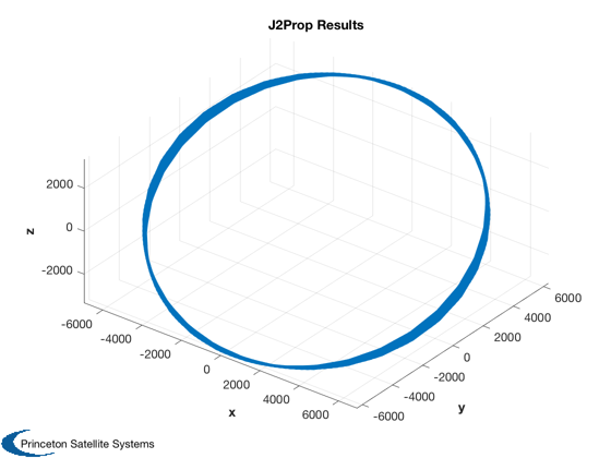
Plot3D(x(1:3,:));
title('J2Prop Results')

Propagate using J2Prop (FOrbCartH):
Elapsed time is 0.381965 seconds.

Compare to analytic

disp('Compare to analytic solution using J2OrbitEffects:')
elFinal   = RV2El(rP(:,end),vP(:,end));
[~, WDot] = J2OrbitEffects( el0(1), el0(5), el0(2), abs(gM.j(2)), gM.mu, gM.a );
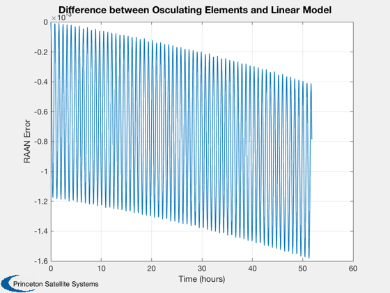
err = (el0(3) + WDot*time(end)) - elFinal(3)

els = RVSet2El( rP, vP, gM.mu );

[tP,tL] = TimeLabl( time );
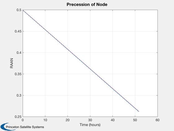
Plot2D(tP,els(:,3)',tL,'RAAN','Precession of Node')
hold on
plot(tP,el0(3)+WDot*time,'r')
Plot2D(tP,els(:,3)'-(el0(3)+WDot*time),tL,'RAAN Error',...
  'Difference between Osculating Elements and Linear Model')

Compare to analytic solution using J2OrbitEffects:
err =
   0.00078836

Try with less points

RK45 will produce an error if the integration tolerance can't be met - i.e. not enough points.

disp('Show that RK45 is sensitive to number of points:')
nPts2 = 200;
try
  time2 = linspace(0,dur,nPts2);
  x2 = J2Prop( [r;v], jD0, time2, gM );
catch exception
  disp('Whoops!')
  disp(exception.message)
end

Show that RK45 is sensitive to number of points:
Whoops!
Exceeded the max error count of 10. Try reducing your stepsize and running again.
h =   9.3725e+01, hMax =   9.3725e+02, error =   1.5134e-05, tau =   2.4625e-06

Try with more points

How does it compare to the analytic solution now? Perhaps "better" but 1000 points was certainly sufficient.

disp('Add points and try again:')
nPts3   = 3000;
time3   = linspace(0,dur,nPts3);
tic
x3      = J2Prop( [r;v], jD0, time3, gM );
toc
elF3    = RV2El(x3(1:3,end),x3(4:6,end));
err3    = (el0(3) + WDot*time3(end)) - elF3(3);
fprintf('Yes, just a little closer with %d points\n',nPts3)
[err err3]


%--------------------------------------

Add points and try again:
Elapsed time is 0.638075 seconds.
Yes, just a little closer with 3000 points
ans =
   0.00078836   0.00071956