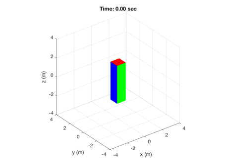
Demonstrates rigid body rotation.

You enter a time step, end time, dimensions of the cube and mass.
You can also enter a step body fixed disturbance.

The displayed cube is based on the entered dimensions.
During the simulation you can rotate the cube with the mouse.

Uses the SCT functions:

Inertias
AnimateCube
RK4 (Runge-Kutta 4th order numerical integration)
FRB (rigid body rhs)
TimeLabl (generates reasonable labels in sec, min, etc.)
Plot2D
Plot3D
------------------------------------------------------------------------
See also AnimateCube, Inertias, QTForm, Figui, Plot2D, Plot3D,
TimeLabl, Mag, RK4
------------------------------------------------------------------------

Contents

%-------------------------------------------------------------------------------
%   Copyright (c) 1995-2006 Princeton Satellite Systems, Inc.
%   All rights reserved.
%-------------------------------------------------------------------------------

The integration time step (seconds)

%--------------------------
dT   = 0.2;
tEnd = 100;

Spacecraft Properties (select a set of xYZ dimensions below)

%----------------------
xYZ  = [1 1   4]; % m  (slight wobble)
%xYZ  = [1 1 1/4]; % m  (very stable)
%xYZ  = [1 1  40]; % m  (unstable, enters a flat spin)
mass = 1000; % kg

Initial conditions [quaternion;rate]

%-------------------------------------
q0 = [1;0;0;0];
w0 = [0.01;0.01;0.1];
x  = [q0;w0];

Step disturbances

%----------------------
tDist = [0.0;0.0;0.0];

Number of sim steps

%--------------------
nSim = tEnd/dT;
t    = dT:dT:tEnd;

Spacecraft Inertia

%--------------------
inr    = Inertias( mass, xYZ, 'box', 1 );
invInr = inv(inr);

Plotting array

%---------------
xPlot = zeros(7,nSim);

Initialize the animation

%-------------------------
tag = AnimateCube( 'initialize', xYZ );

Run the simulation

%-------------------
for k = 1:nSim

  % Store the current state for plotting
  %-------------------------------------
  xPlot(:,k) = x;

  % Update the animation
  %---------------------
  %AnimateCube( 'update', tag, [x(1:4);t(k)] );
  %pause(dT/2)

  % Integrate
  %----------
  x = RK4('FRB',x,dT,0,inr,invInr,tDist);

end

playback = @(x) AnimateCube( 'update', tag, [xPlot(1:4,fix(x/dT)+1);t(fix(x/dT)+1)] );
PlaybackControls( 0, tEnd, 0, playback, dT, 'NutationAnimation' )

2D Plots

%---------
% Scale the time from seconds
[t, tL] = TimeLabl( (0:(nSim-1))*dT );
% Make the 2D time history plots
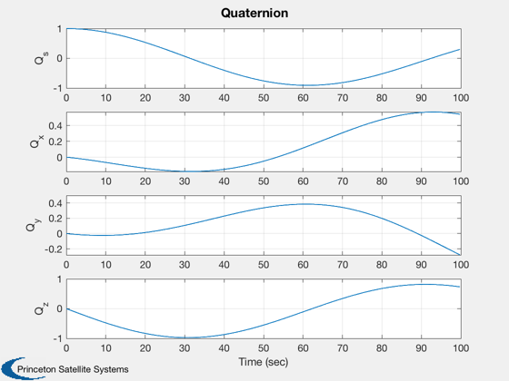
Plot2D(t,xPlot( 1: 4,:),tL,['Q_s';'Q_x';'Q_y';'Q_z'],'Quaternion')
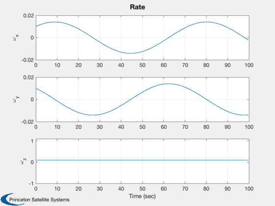
Plot2D(t,xPlot( 5: 7,:),tL,['\omega_x';'\omega_y';'\omega_z'],'Rate')

3D Plot

%--------
% The x-axis
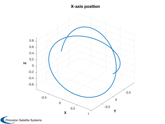
u = [1;0;0];
% Transform to ECI
r = QTForm( xPlot(1:4,:), u );
% Create the 3D plot
Plot3D( r, 'X', 'Y', 'Z', 'X-axis position' )

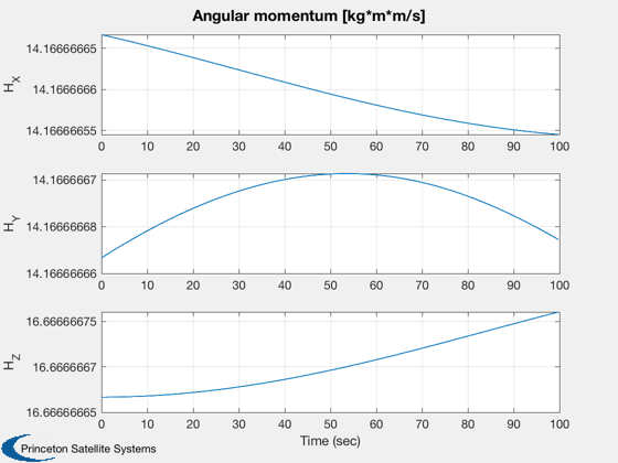
Analyze Angular Momentum

%-------------------------
H = zeros(3,nSim);
q = xPlot(1:4,:);
w = xPlot(5:7,:);
for i=1:nSim
   H(:,i) = QTForm(q(:,i),inr*w(:,i));
end
Plot2D( t, H, tL, ['H_X';'H_Y';'H_Z'], 'Angular momentum [kg*m*m/s]');
% Print the angular momentum info
fprintf('\nAngular Momentum\n================\n');
fprintf('\n\tMean:    \t%f\n\tVariance:\t%g\n\n',mean(Mag(H)),var(Mag(H)))

Angular Momentum
================

	Mean:    	26.060826
	Variance:	2.50924e-19

Create an index to the plots

%-----------------------------
Figui;


%--------------------------------------

Published with MATLAB® R2019a