Contents
CMG demo
This tests the dynamics with 3 CMGs.
It looks at angular momentum conservation and looks for a symmetric inertia matrix
------------------------------------------------------------------------
See also: RHSCMG, StepTorque, RK4, TimeLabl, Plot2D, NewFig, Figui
------------------------------------------------------------------------
%--------------------------------------------------------------------------
%   Copyright (c) 2020 Princeton Satellite Systems, Inc.
%   All rights reserved.
%--------------------------------------------------------------------------
%   Since version 2020.2
%--------------------------------------------------------------------------
User inputs
Simulation control
dT        = 0.1;
tEnd      = 100;

% Disturbance torque
torque    = [0;0;0];

% Core attitude states
q         = [1;0;0;0];  % Quaternion
omega     = [0.01;0.2;0.01]; % Angular rate

% Wheel and gimbal rates
wGW       = 0.1*rand(6,1);
Initialize the simlation
x         = [q;0;0;0;omega;wGW];

% Storage for plots
n         = ceil(tEnd/dT);
xP        = zeros(length(x)+4,n+1);

% Get default data structure
d                   = RHSCMG;
d.fDist             = @StepTorque;  % Disturbance function pointer
d.torqueDisturbance = torque;
t                   = 0;

% Get the initial momentum
[~,~,h0]            = RHSCMG(x,t,d);
Simulation loop using 4th order Runge-Kutta
for k = 1:n

  % Control
  d.torqueG = [0;0;0];
  d.torqueW = [0;0;0];

  % For plotting
  [~,inr,h] = RHSCMG(x,t,d);
	inrErr    = max(max(abs(inr - inr')));
  xP(:,k)   = [x;h-h0;inrErr];

  % Passes a pointer to RHSRigidBody for numerical integration
  x         = RK4(@RHSCMG,x,dT,t,d);
  t         = t + dT;
end

% Last point for plotting
[~,inr,h]	= RHSCMG(x,t,d);
inrErr    = max(max(abs(inr - inr')));
xP(:,n+1) = [x;h-h0;inrErr];

% Reduce the time step
dT2         = dT/1000;

% Storage for plots
n2          = ceil(tEnd/dT);
xP2         = zeros(3,n2+1);

x         = [q;0;0;0;omega;wGW];
Simulation loop using 4th order Runge-Kutta with a smaller time step
for k = 1:n2

  % Control
  d.torqueG = [0;0;0];
  d.torqueW = [0;0;0];

  % For plotting
  [~,~,h]   = RHSCMG(x,t,d);
  xP2(:,k)  = h-h0;

  % Passes a pointer to RHSRigidBody for numerical integration
  x         = RK4(@RHSCMG,x,dT2,t,d);
  t         = t + dT2;
end

% Last point for plotting
[~,~,h]	= RHSCMG(x,t,d);
xP2(:,n+1) = h-h0;
Plotting
tSec = (0:n)*dT;
[t,tL] = TimeLabl(tSec);
yL = [d.states(:)' {'\Delta H_x (Nms)'} {'\Delta H_y (Nms)'} {'\Delta H_z (Nms)'} {'\Delta I (kg-m^2)'}];
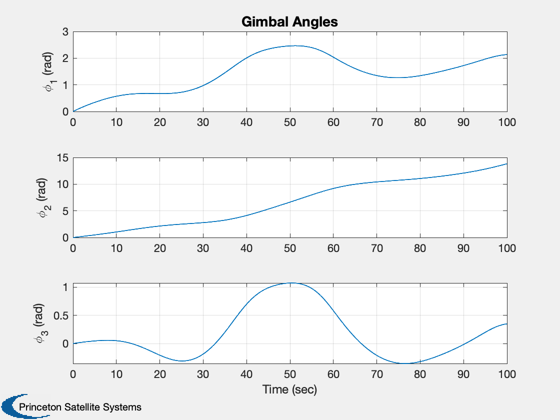
k = 5:7;
Plot2D(t,xP(k,:),tL,yL(k),'Gimbal Angles')
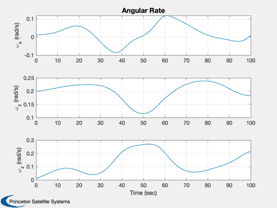
k = 8:10;
Plot2D(t,xP(k,:),tL,yL(k),'Angular Rate')
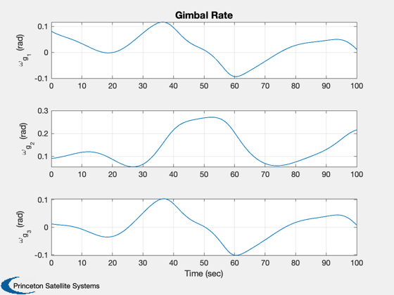
k = 11:13;
Plot2D(t,xP(k,:),tL,yL(k),'Gimbal Rate')
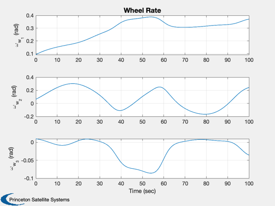
k = 14:16;
Plot2D(t,xP(k,:),tL,yL(k),'Wheel Rate')
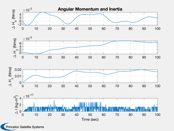
k = 17:20;
Plot2D(t,xP(k,:),tL,yL(k),'Angular Momentum and Inertia')
k = 17:19;
tSec = (0:n2)*dT;
[t2,tL] = TimeLabl(tSec);
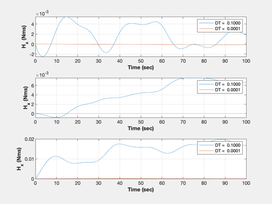
dTL = sprintf('DT = %7.4f',dT);
dTL2 = sprintf('DT = %7.4f',dT2);
NewFig('Angular Momentum')
subplot(3,1,1)
plot(t,xP(17,:))
hold on
plot(t2,xP2(1,:));
grid on
XLabelS(tL);
YLabelS('H_x (Nms)');
legend(dTL,dTL2);
subplot(3,1,2)
plot(t,xP(18,:))
hold on
plot(t2,xP2(2,:));
grid on
XLabelS(tL);
YLabelS('H_x (Nms)');
legend(dTL,dTL2);
subplot(3,1,3)
plot(t,xP(19,:))
hold on
plot(t2,xP2(3,:));
grid on
XLabelS(tL);
YLabelS('H_x (Nms)');
legend(dTL,dTL2);
Figui
%--------------------------------------