Demonstrate computing angles for a sail with a pair of vanes.

Explore effects of sail cone angle on vane control output. Uses a 2 vane example (PlateWithVanes).

Since version 9.
------------------------------------------------------------------------
See also SolveVaneAngles, SailDisturbance, Theta0, DrawSCPlanPlugIn,
Cone, Constant, InformDlg, NewFig, Plot2D, TitleS, XLabelS, YLabelS, Unit,
Date2JD, El2RV, ConeClockToU, QSail, DisturbanceStruct, EnvironmentStruct,
ProfileStruct, SailEnvironment, CP1Props, UpdateSailOpticalProps,
ApplyProfileToModel, SailPropsToAccel
------------------------------------------------------------------------

Contents

%-------------------------------------------------------------------------------
%	 Copyright 2009 Princeton Satellite Systems, Inc.
%  All rights reserved.
%-------------------------------------------------------------------------------

Set up the problem

%--------------------
clear SailDisturbance

Use a CAD model to get actual torque produced by vanes

%-------------------------------------------------------
g = load('PlateWithVanes');

Define spacecraft properties

%-----------------------------
mass  = g.mass.mass; % spacecraft mass in kg
lSail = max(max(g.component(2).v)); % sail length along one side in m
area  = sum(g.component(2).a);
acc0  = SailPropsToAccel( area, mass );

Vane area

%-------------
areaVane = g.component(3).a; % m2

Maximum torque

%---------------
thetaMax = 80*pi/180;
Ps       = Constant('solar pressure mks');
fVane    = 2*Ps*areaVane;
Tmax     = 2*lSail*fVane*sin(thetaMax);

Environment and disturbance models

%-----------------------------------
d = struct;
d = EnvironmentStruct( d );
d = DisturbanceStruct( d );
d.aeroOn   = 0;
d.albedoOn = 0;
d.magOn    = 0;
d.radOn    = 0;

Profile: orbit, attitude

%-------------------------
jD    = Date2JD;
[r,v] = El2RV([Constant('au') 0 0 0 0 0],[],Constant('mu sun'));
uSun  = -Unit(r);
qS    = QSail( uSun, r, v );
p    = ProfileStruct;
p.q  = qS;
p.r  = r;
p.v  = v;
p.jD = jD;
% states for rotating vanes
p.body  = [2 3];
p.angle = [0; 0];
p.axis  = [0 0 1; 0 0 1]';

Environment will be constant over this short period

%----------------------------------------------------
env = SailEnvironment( 'sun', p, d );

Compute full disturbances for different vane angles and sail attiude

%----------------------------------------------------------------------
disp('Sail vanes demo ----------------------')

% Disturbances
[f, tq] = SailDisturbance( g, p, env, d );
disp('Torque for all zero angles - should be zero!')
tq.total

% Now rotate the vanes with the sail straight-on to the sun
p.angle = [20; 20]*pi/180;
[f, tq] = SailDisturbance( g, p, env, d );
disp('Torque for vanes angles of 20 degrees - pure roll torque')
tq.total

% Next give the sail a cone angle - see torques in other axes
cone = pi/6;
clock = 0;
[u,qItoCC] = ConeClockToU( cone, clock, qS );
p.q  = qItoCC;
[f, tq] = SailDisturbance( g, p, env, d );
disp('Torque for vanes angles of 20 degrees with cone angle of 30 degrees;')
disp('no longer a pure roll torque but evenly distributed in two axes.')
tq.total

% Now give the sail a clock angle - no change
clock = pi/4;
[u,qItoCC] = ConeClockToU( cone, clock, qS );
p.q  = qItoCC;
[f, tq] = SailDisturbance( g, p, env, d );
disp('Clock angle doesn''''t change the body torques')
tq.total

% Investigate the effect of cone angle on the three-axis torque produced

Sail vanes demo ----------------------
Torque for all zero angles - should be zero!
ans =
  -9.5352e-18
   1.3878e-17
   7.5266e-17
Torque for vanes angles of 20 degrees - pure roll torque
ans =
      0.21871
            0
   7.4593e-17
Torque for vanes angles of 20 degrees with cone angle of 30 degrees;
no longer a pure roll torque but evenly distributed in two axes.
ans =
       0.1718
      0.19171
   -0.0032355
Clock angle doesn''t change the body torques
ans =
       0.1718
      0.19171
   -0.0032355

(Vanes don't produce a pure roll torque for nonzero cone angle)

%-----------------------------------------------------------------------
cones = linspace(0,pi/4,50);
clock = 0;
vanes = [10;20;30;40;50;65;80];
zz      = zeros(length(vanes),length(cones));
torqueX = zz;
torqueY = zz;
torqueZ = zz;
for k = 1:length(cones)
  [u,qItoCC(:,k)] = ConeClockToU( cones(k), clock, qS );
  p.q  = qItoCC(:,k);
  for j = 1:length(vanes)
    p.angle = vanes(j)*[1; 1]*pi/180;
    [f, tq] = SailDisturbance( g, p, env, d );
    torqueX(j,k) = tq.total(1);
    torqueY(j,k) = tq.total(2);
    torqueZ(j,k) = tq.total(3);
  end
end
conePlot = cones*180/pi;

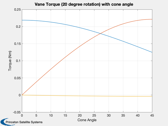
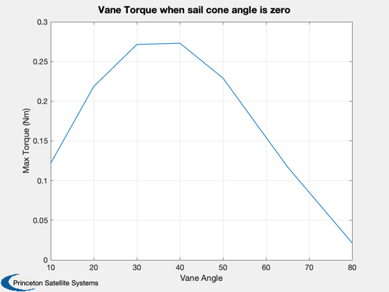
Plot the curves for a single vane angle and all cone angles

%------------------------------------------------------------
% Nominal curves, at 20 degrees
Plot2D(conePlot,[torqueX(2,:);torqueY(2,:);torqueZ(2,:)],'Cone Angle','Torque (Nm)','Vane Torque (20 degree rotation) with cone angle')
% Confirm typical magnitude curve when cone is zero
Plot2D(vanes',torqueX(:,1)','Vane Angle','Max Torque (Nm)','Vane Torque when sail cone angle is zero')

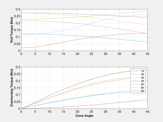
Plot the torque profiles in each axis

%--------------------------------------
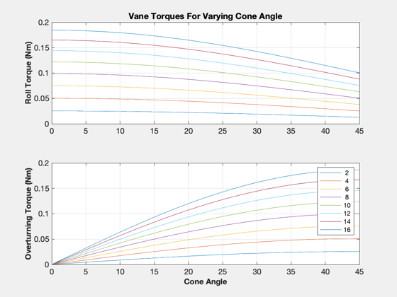
NewFig('Torque Profiles')
TitleS('Vane Torques For Varying Cone Angle')
subplot(2,1,1)
plot(conePlot,torqueX)
YLabelS('Roll Torque (Nm)')
grid on
subplot(2,1,2)
plot(conePlot,torqueY)
grid on
YLabelS('Overturning Torque (Nm)')
XLabelS('Cone Angle')
legH = legend(num2str(vanes));
set(legH,'fontsize',9)

Redo above analysis with a smaller set of vane angles

%-------------------------------------------------------
clock = 0;
vanes = 2:2:16;
torqueX = zz;
torqueY = zz;
torqueZ = zz;
for k = 1:length(cones)
  p.q  = qItoCC(:,k);
  for j = 1:length(vanes)
    p.angle = vanes(j)*[1; 1]*pi/180;
    [f, tq] = SailDisturbance( g, p, env, d );
    torqueX(j,k) = tq.total(1);
    torqueY(j,k) = tq.total(2);
    torqueZ(j,k) = tq.total(3);
  end
end

% This figure shows that when the sail has an angle to the sun, and the
% vanes have equal angles, an overturning torque is produced in addition to
% the roll torque. This is because the vanes have different apparent areas

to the sun.

%--------------------------------------------------------------------------
NewFig('Torque Profiles')
subplot(2,1,1)
plot(conePlot,torqueX)
grid on
YLabelS('Roll Torque (Nm)')
TitleS('Vane Torques For Varying Cone Angle')
subplot(2,1,2)
plot(conePlot,torqueY)
grid on
YLabelS('Overturning Torque (Nm)')
XLabelS('Cone Angle')
legH = legend(num2str(vanes'));
set(legH,'fontsize',9)

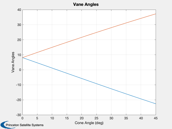
Investigate differential vane commanding for pure roll torque

To achieve a pure roll torque with varying sail cone angle we have to command the vanes to different angles. SolveVaneAngles uses Newton's method with a numerical Jacobian to find the combination of vane angles

that gives the desired torque.

%---------------------------------------------------
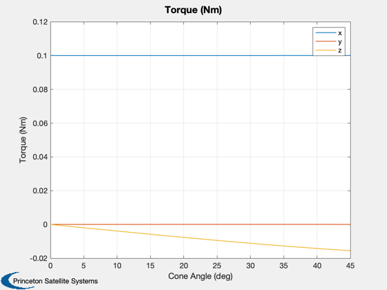
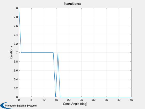
Tcommand = [0.1; 0];
% Nominal angle for roll torque, for initialization
theta0 = asin(Tcommand(1)./(2*lSail*fVane));
theta = [theta0;theta0];
% Initialize plot matrices
torqueSolved = zeros(3,length(cones));
thetas       = zeros(2,length(cones));
ks           = zeros(1,length(cones));
% Informational window
iH = InformDlg( 'Running loop of SolveVaneAngles...', 'SailVanesDemo' );
for k = 1:length(cones)
  p.q  = qItoCC(:,k);
  [theta,iter] = SolveVaneAngles( Tcommand, theta, g, env, p, d );
  p.angle = theta;
  [f, tq] = SailDisturbance( g, p, env, d );
  torqueSolved(:,k) = tq.total;
  thetas(:,k) = theta;
  ks(k) = iter;
end
close(iH)

% See that the average angle remains the same and pure roll torque is
% achieved. The number of iterations to meet the tolerance is shown.
%

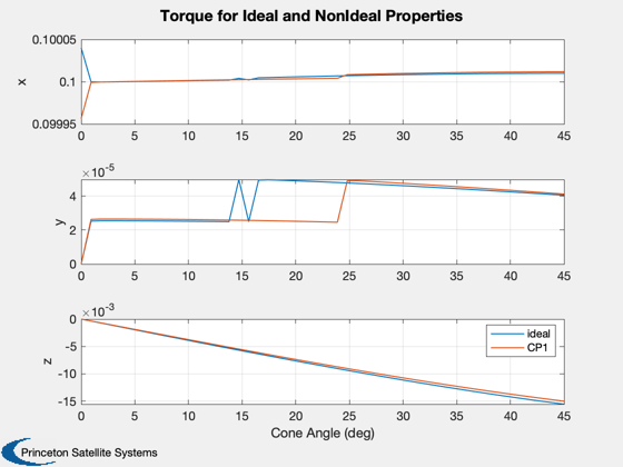
A small torque is generated in the 3rd axis, increasing with cone angle.

%-------------------------------------------------------------------------
Plot2D(conePlot,thetas*180/pi,'Cone Angle (deg)','Vane Angles')
Plot2D(conePlot,torqueSolved,'Cone Angle (deg)','Torque (Nm)')
legend('x','y','z')
Plot2D(conePlot,ks,'Cone Angle (deg)','Iterations')

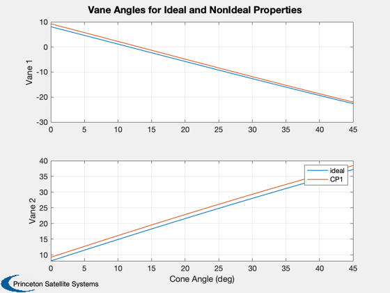
Redo angle solving with non-ideal optical properties

%-----------------------------------------------------
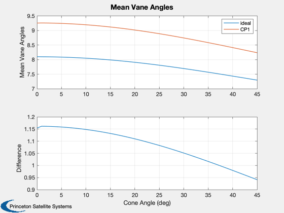
[optical, infrared, thermal] = CP1Props;
g2 = UpdateSailOpticalProps( g, optical, thermal, infrared );
% Reinitialize angles for solver
theta = [theta0;theta0];
% Clear disturbances of ideal model
clear SailDisturbance
% Informational window
iH = InformDlg( 'Running loop of SolveVaneAngles...', 'SailVanesDemo' );
torqueSolved2 = zeros(3,length(cones));
thetas2       = zeros(2,length(cones));
ks2           = zeros(1,length(cones));
for k = 1:length(cones)
  p.q  = qItoCC(:,k);
  [theta,iter] = SolveVaneAngles( Tcommand, theta, g2, env, p, d );
  p.angle = theta;
  [f, tq] = SailDisturbance( g2, p, env, d );
  torqueSolved2(:,k) = tq.total;
  thetas2(:,k) = theta;
  ks2(k) = iter;
end
close(iH)

Plot2D(conePlot,[thetas*180/pi;thetas2*180/pi],'Cone Angle (deg)',{'Vane 1','Vane 2'},...
  'Vane Angles for Ideal and NonIdeal Properties','lin',{[1 3],[2 4]})
legend('ideal','CP1')
Plot2D(conePlot,[torqueSolved;torqueSolved2],'Cone Angle (deg)',{'x','y','z'},...
  'Torque for Ideal and NonIdeal Properties','lin',{[1 4],[2 5],[3 6]})
legend('ideal','CP1')

% Compare mean and offset angles for two cases. Mean angle is NOT constant.
% The different in the mean angles for nonideal properties is over 1

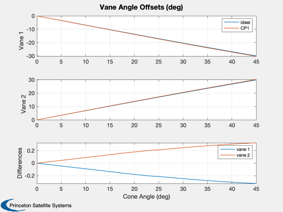
degree, while for the offset angles it is less than 0.5 degree.

%--------------------------------------------------------------------------
m1 = sum(thetas)/2;
m2 = sum(thetas2)/2;
d1 = thetas - repmat(m1,2,1);
d2 = thetas2 - repmat(m2,2,1);
Plot2D(conePlot,[m1;m2;m2-m1]*180/pi,'Cone Angle (deg)',{'Mean Vane Angles','Difference'},...
  'Mean Vane Angles','lin',{[1 2],3})
subplot(2,1,1)
legend('ideal','CP1')
Plot2D(conePlot,[d1;d2;d2-d1]*180/pi,'Cone Angle (deg)',{'Vane 1','Vane 2','Differences'},...
  'Vane Angle Offsets (deg)','lin',{[1 3],[2 4],[5 6]})
legH = legend('vane 1','vane 2');
set(legH,'fontsize',9)
subplot(3,1,1)
legH = legend('ideal','CP1');
set(legH,'fontsize',9)

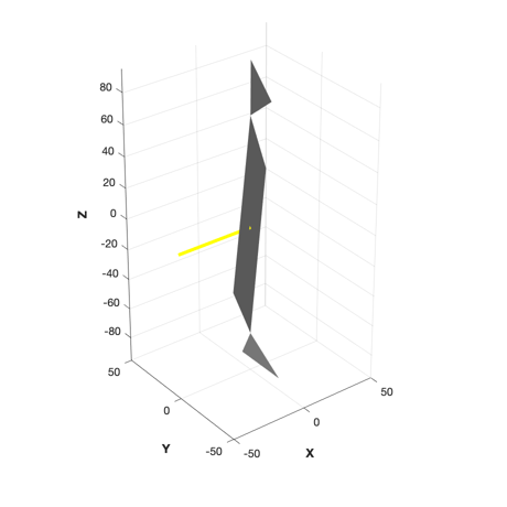
Animate angles (ideal case) using DrawSCPlanPlugIn

%---------------------------------------------------
tag = DrawSCPlanPlugIn( g );
light('position',uSun)
hold on;
plot3([0 g.radius*uSun(1)],[0 g.radius*uSun(2)],[0 g.radius*uSun(3)],'y','linewidth',3)
p.q = qItoCC;
p.angle = thetas;
for k = 1:length(cones)
  g = ApplyProfileToModel( g, p, k );
  DrawSCPlanPlugIn( 'update', tag, g )
  pause(0.4)
end

%--------------------------------------

Published with MATLAB® R2020a