Demonstrate gimballed boom control.

This demo uses the PlateWithBoom CAD model. The gimbals have a
1-2 sequence, first around the X axis and then around the Y axis.
The control law is designed using PIDMIMO. There is no roll
actuation and therefore the attitude trajectory must use
only Y and Z torques.

The attitude dynamics assume fixed gimbal rates.
The CAD model is a perfectly specular plate with a control boom.

Functions demonstrated:
    PIDMIMO
    ConeClockToQConstrained
    HGimballedBoom
    TwoBodyRateModel
    SailDisturbance

Since version 7.
------------------------------------------------------------------------
See also BoomActuation, which rotates the gimbals without following   a
specific control law., AC, ACPlot, CrossSection, DrawSCPlanPlugIn,
PIDMIMO, QForm, QMult, QPose, QTForm, Constant, WaitBarManager, Plot2D,
TimeLabl, Mag, RK4, Unit, JD2000, El2RV, Accel, GimbalRates,
HGimballedBoom, ConeClockToQConstrained, QSail, QToConeClock,
HingeRotationMatrix, ProfileStruct, SailDisturbance, SailEnvironment
------------------------------------------------------------------------

Contents

%-------------------------------------------------------------------------------
%	Copyright (c) 2005,2006 Princeton Satellite Systems, Inc.
%   All rights reserved.
%-------------------------------------------------------------------------------

%%%%%%%%%%%%%%%%%%%%%%%%%%%%%%%%%%%%%%%%%%%%%%%%
% User Parameters
%%%%%%%%%%%%%%%%%%
% Change these to explore the system dynamics.
%%%%%%%%%%%%%%%%%%%%%%%%%%%%%%%%%%%%%%%%%%%%%%%%
% Commanded cone and clock angles (rad)
coneCommand = 0; %0.5;
clockCommand = 0; %0.1;
% Initial cone and clock angles (rad)
cone0 = 0.1; %0.5;
clock0 = 0.0;
% Nominal gimbal rate (rad/s)
aRateNom = 0.3;
% Controller natural frequency (rad/sec)
wn = 0.0001;
% Maximum angular change for new target (rad)
deltaAngle = 0.2;
% Duration for sim (s)
tDuration = 12000;
%%%%%%%%%%%%%%%%%%%%%%%%%%%%%%%%%%%%%%%%%%%%%%%%

Clean up workspace

%-------------------
clear SailDisturbance

%---------------------------------

Load the control boom sail model

%---------------------------------
g = load('PlateWithBoom.mat');
%g.mass.inertia(1,1) = g.mass.inertia(2,2);
% To view the model, run: DrawSCPlanPlugIn( 'initialize', g );

Sim timing

%-----------
dTo  = floor(2*pi/wn/100); % sec, outer dT for ACS
dTi  = dTo/10;              % sec, inner dT for boom control via gimbals
nSim = floor(tDuration/dTi);

%---------------------------------------------------------

Control parameters - use PIDMIMO to design control loops

%---------------------------------------------------------
aNom         = aRateNom*ones(2,1);
xN           = zeros(6,1);      % Controller state
inr          = diag([1 1 1]);   % Unit inertia
zeta         = 3;               % Damping ratio
tauInt       = 2*pi/zeta/wn;            % Integrator time constant
omegaR       = 5*wn;           % Rate filter frequency
sType        = 'z';             % Type of equations
[aC, bC, cC, dC] = PIDMIMO( inr, zeta*ones(1,3), wn*ones(1,3), tauInt*ones(1,3), ...
                            omegaR*ones(1,3), dTo, sType );
% Resulting control values are accelerations (due to unit inertia input).
% Will multiply by full inertia to compute torque.

Sail physical parameters

%-------------------------
aSail = CrossSection(g);
Ps    = 1367/3e8;
fSail = 2*Ps*aSail*[-1;0;0];       % Specular reflective force in body frame, N
aBoom(:,1) = Cross([0;1;0],fSail); % Boom control axes
aBoom(:,2) = Cross([0;0;1],fSail);
mC      = g.body(1).mass.mass;     % Core is body 1
mB      = g.body(2).mass.mass;     % Boom is body 2
rBoomCM = Mag(g.body(2).mass.cM);  % Distance to boom center-of-mass

%-------------------------------

Create the disturbance profile

%-------------------------------

Initial Julian date

%--------------------
p          = ProfileStruct;
p.jD       = JD2000;

% Parameters for the orbit.

We are creating a circular heliocentric orbit.

%-----------------------------------------------
r   = Constant('au'); % Radius in km
mu  = Constant('mu sun');
el  = [r 0 0 0 0 0];

Orbit state

%------------
[p.r,p.v]  = El2RV(el,[],mu);

Initial Quaternion (inertial to body frame)

%--------------------------------------------
q0  = ConeClockToQConstrained(cone0,clock0,p.r,p.v,-Unit(p.r));
p.q = q0;

% Gimbal angles. The sail is two body with a gimbaled boom.
% The first angle is the one nearest the core.
% The axes correspond to the angles.
% The body array says each gimbal is at the joint between the

core and the boom. The core is defined as body 1 in the CAD file.

%------------------------------------------------------------------
p.angle    = [0;0];
p.axis     = [1 0;0 1;0 0];
p.body     = [2 2];

%--------------------------

Create the data structure

%--------------------------
d          = [];
d.aeroOn   = 0;
d.albedoOn = 0;
d.solarOn  = 1.0;
d.magOn    = 0;
d.radOn    = 0;
d.ggOn     = 1.0;

% Orbiting the sun. SailDisturbance can handle any planet or
% a heliocentric orbit. However, not all planets have magnetic

field models or atmospheric density models.

%-------------------------------------------------------------
d.planet   = 'sun';

Initial state

%--------------
t     = 0;       % time
tO    = dTo;     % Outer timer
w     = [0;0;0]; % body rates
angle = [0;0];   % boom gimbal angles
aDot  = [0;0];   % boom gimbal rates
x     = [p.q;w;angle;aDot];
hW    = [0;0;0]; % stored momentum
alpha = 0;       % initial gimbal angle command
beta  = 0;       % initial gimbal angle command
cM    = [0;0];   % Commanded CM for boom

tPlot  = zeros(1,nSim);
xPlot  = zeros(length(x),nSim);
hPlot  = zeros(3,nSim);  % angular momentum
tqPlot = zeros(6,nSim);  % commanded and achieved torque, stacked
aCPlot = zeros(2,nSim);  % Commanded gimbal angles
aEPlot = zeros(4,nSim);  % Euler angle errors
qSPlot = zeros(4,nSim);  % Quaternion in rotating sail frame
cMPlot = zeros(2,nSim);

Commanded quaternion, inertial to body frame, constant

%-------------------------------------------------------
qC   = ConeClockToQConstrained(coneCommand,clockCommand,p.r,p.v,-Unit(p.r));
uI   = QTForm( qC, [1;0;0] );
sN   = sin(coneCommand);
cN   = cos(coneCommand);
qOld = p.q;

% Quaternion from inertial to the local sail rotating frame, which has:
%    x is towards the sun
%    z is as close to the orbit normal as possible
%    y completes the set

Located at the center of the body frame.

%----------------------------------------------------------------------
qIToSail = QSail( -Unit(p.r), p.r, p.v );

Environment - model as constant over this time period.

%-------------------------------------------------------
e = SailEnvironment( 'sun', p, d );

Simulation loop

%----------------
WaitBarManager( 'initialize', struct('nSamp',nSim,'name','Boom Control Demo') );
for k = 1:nSim

  % Store data in plots
  %--------------------
  tPlot(k)    = t;
  xPlot(:,k)  = x;
  % Sail to body quaternion
  qSPlot(:,k) = QMult(QPose(qIToSail),x(1:4));
  if( qSPlot(1,k) < 0 )
    qSPlot(:,k) = -qSPlot(:,k);
  end

  %--------------------------
  % Compute the disturbances.
  %--------------------------
  [f,tq] = SailDisturbance( g, p, e, d );
  tqPlot(4:6,k) = tq.total;

  %-----------------
  % Boom control
  %-----------------

  % Sign conventions
  %-----------------
  % Keep scalar component of quaternion positive
  if( qC(1) < 0 )
    qC = -qC;
  end
  % Inertial to body quaternion
  qIToB = x(1:4);
  if( qIToB(1) < 0 )
    qIToB = -qIToB;
    xPlot(1:4,k) = qIToB;
  end

  %-------------------------------------------------------------------------
  % Euler angle error in body frame. We are only considering Y and Z errors.
  % Determine from commanded normal in body frame.
  %-------------------------------------------------------------------------
  uSailB = QForm( qIToB, uI );
  errY   = uSailB(3);
  errZ   = -uSailB(2);
  eulErr = [errY;errZ];

  %-----------------------------------------------------
  % Outer loop: Update the boom command at dTo intervals
  %-----------------------------------------------------
  if (tO >= dTo)
    % Small angle convention
    %-----------------------
    angleError = [0;eulErr];
    if (Mag(angleError) > deltaAngle)
      angleError = sign(angleError).*min([abs(angleError) [0;[1;1]*deltaAngle]],[],2);
    end

    % Control law and torque
    %-----------------------
    % first compute body acceleration
    accel = cC*xN + dC*angleError;
    % controller state update
    xN    = aC*xN + bC*angleError;
    % convert acceleration to control torque using actual vehicle inertia
    tExt  = -g.mass.inertia*accel;

    % Cp/Cm offset
    %-------------
    % use pinv to allocate torque to controllable axes (Y/Z).
    % assume Cp is at center and compute new Cm from torque and masses.
    cM  = -pinv(aBoom)/cos(cone0)^2*tExt/(mB/(mC+mB));
    mCM = Mag(cM);
    if (mCM >= rBoomCM)
      % requesting CM beyond reach of boom
      % may update to different constraint in future (i.e. angles)
      hB = 0;
    else
      % Boom unit vector component along normal
      hB = sqrt(rBoomCM^2 - mCM^2);
    end
    % New boom unit vector in body frame
    uB = Unit([hB;cM]);

    % Gimbal angles (12 sequence)
    %----------------------------
    % Rotations are defined as:
    % uB = C1(alpha)*C2(beta)*[1;0;0], or
    % uB = Eul2Mat([alpha;beta;0])*[1;0;0]
    alpha = atan2(uB(2),-uB(3));
    beta  = acos(uB(1));

    % Reset outer timer
    %------------------
    tO = 0;
  end

  % Inner loop: drive gimbals to commanded location
  %------------------------------------------------
  [aDot,angleCommand] = GimbalRates( x(8:9), [alpha;beta], aNom, dTi );

  % Store commanded torque and angles
  %----------------------------------
  aEPlot(1:2,k) = eulErr;          % store actual Euler errors
  aEPlot(3:4,k) = angleError(2:3); % limited angle error
  aCPlot(:,k)   = angleCommand;
  tqPlot(1:3,k) = tExt;
  cMPlot(:,k)   = cM;

  %-------------
  % RHS
  %-------------
  % x = [q;omega;gimbal angles;gimbal rates]
  % Use zeros as placeholders for orbit state (not used)
  [hPlot(:,k), hW] = HGimballedBoom( [zeros(6,1);x], g, p.axis, aDot, hW );
  x(10:11) = aDot;

  % Integrate
  %----------
  x = RK4( 'TwoBodyRateModel', x, dTi, t, f, tq, g, p, hW );

  % Update profiles
  %----------------
  t    = t + dTi;
  tO   = tO + dTi;
  p.jD = p.jD + dTi/86400;
  p.q  = x(1:4,:);
  p.angle = x(8:9);

  WaitBarManager( 'update', k ); drawnow;

end
WaitBarManager( 'close' );

Prepare data for plotting

%--------------------------
%Plot2D(tPlot,hPlot,[],[],'Inertial Angular Momentum')
% Commanded sail to body quaternion
qSC = QMult(QPose(qIToSail),qC);
if qSC(1) < 0
  qSC = -qSC;
end
qCPlot = repmat(qSC,1,nSim);
[coneP,clockP] = QToConeClock(xPlot(1:4,:),repmat(p.r,1,nSim),repmat(p.v,1,nSim),...
  -repmat(Unit(p.r),1,nSim));
[tPlot2, tLabl] = TimeLabl( tPlot );

h = [];
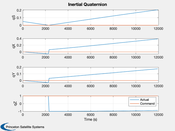
h(1) = Plot2D(tPlot,[xPlot(1:4,:);repmat(qC,1,nSim)],'Time (s)',{'qS','qX','qY','qZ'},'Inertial Quaternion',[],[1 5; 2 6; 3 7; 4 8]);
legend('Actual','Command')
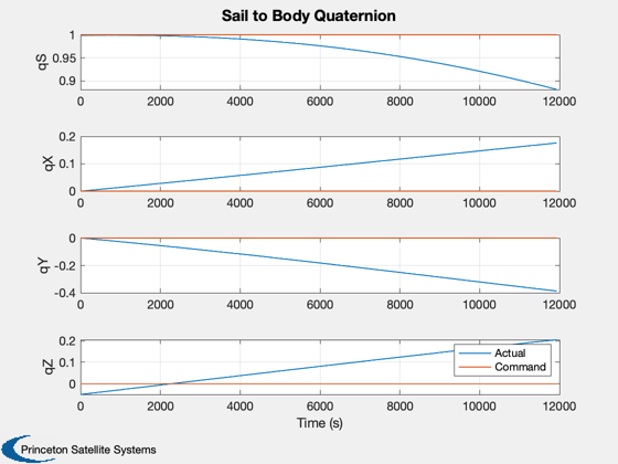
Plot2D(tPlot,[qSPlot;qCPlot],'Time (s)',{'qS','qX','qY','qZ'},'Sail to Body Quaternion',[],[1 5; 2 6; 3 7; 4 8]);
legend('Actual','Command')
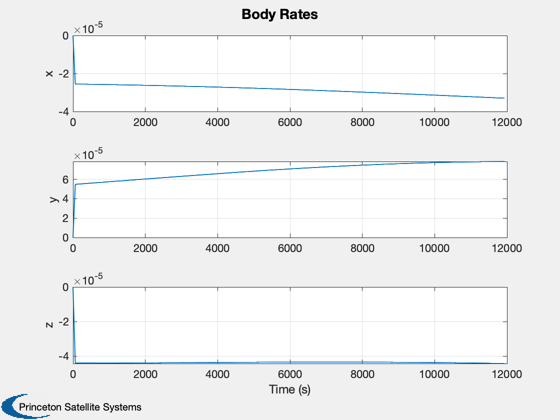
h(2) = Plot2D(tPlot,xPlot(5:7,:),'Time (s)',{'x','y','z'},'Body Rates');
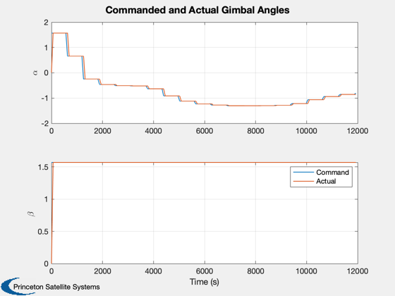
h(3) = Plot2D(tPlot,[aCPlot;xPlot(8:9,:)],'Time (s)',{'\alpha','\beta'},'Commanded and Actual Gimbal Angles',[],{[1 3],[2 4]});
legend('Command','Actual')
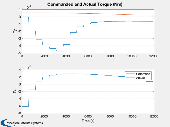
h(4) = Plot2D(tPlot,tqPlot,'Time (s)',{'Ty','Tz'},'Commanded and Actual Torque (Nm)',...
           [],{[2 5],[3 6]});
legend('Command','Actual')
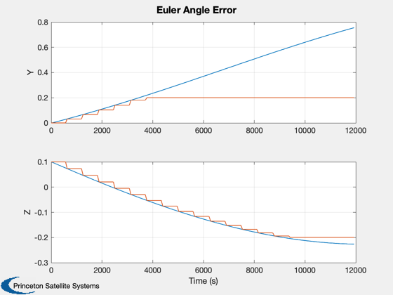
Plot2D(tPlot,aEPlot,'Time (s)',{'Y','Z'},'Euler Angle Error','lin',{[1 3] [2 4]});

% Commanded boom CM control
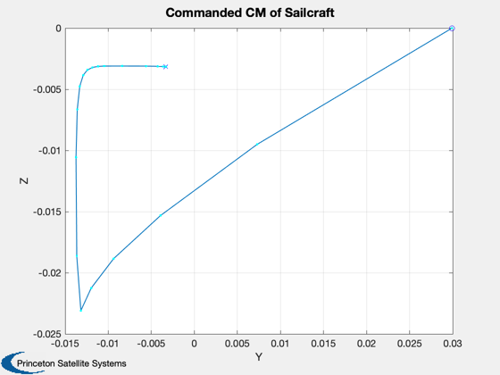
Plot2D(cMPlot(1,:),cMPlot(2,:),'Y','Z','Commanded CM of Sailcraft');
hold on
plot(cMPlot(1,1),cMPlot(2,1),'bo');
plot(cMPlot(1,end),cMPlot(2,end),'bx');
plot(cMPlot(1,:),cMPlot(2,:),'c.');

Try plotting cone/clock angles

%-------------------------------
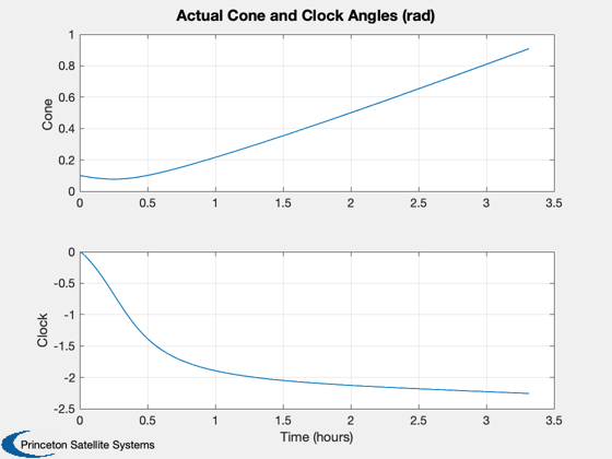
Plot2D(tPlot2,[coneP;clockP], tLabl, {'Cone','Clock'}, 'Actual Cone and Clock Angles (rad)')

if (0)
  % Save plots for use in user's guide.
  c   = cd;
  dBC = fileparts(which('BoomControl'));
  cd(dBC)
  print(h(1),'-depsc2','BCQuaternion')
  print(h(2),'-depsc2','BCRates')
  print(h(3),'-depsc2','BCAngles')
  print(h(4),'-depsc2','BCTorque')
end

% Animate resulting sail and boom motion
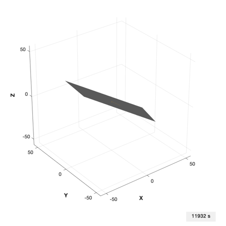
tag = DrawSCPlanPlugIn( 'initialize', g );
nO = floor(dTo/dTi);
nAnim = floor(0.5*nSim/nO);
kAnim = 1:nAnim:nSim;
u = uicontrol('style','text','string','0 s','position',[380 10 60 20]);
yA = g.radius*[-1 1 -1 1 -1 1];
for k = kAnim
  g.body(1).bHinge.q = qSPlot(1:4,k);
  % TBD: add boom motion (bHinge of inner body)
  bBoomToCore = HingeRotationMatrix( xPlot(8:9,k), [1 0;0 1;0 0] )';
  g.body(2).bHinge.b = bBoomToCore;
  DrawSCPlanPlugIn( 'update', tag, g );
  axis(yA);
  set(u,'string',[num2str(k*dTi) ' s'])
  drawnow;
  pause(0.2);
end


%--------------------------------------
% PSS internal file version information
%--------------------------------------

Published with MATLAB® R2020a