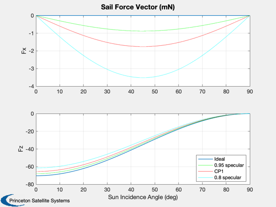
Compare the solar pressure force for ideal and nonideal circular sails.

Compare an ideal, perfectly specular sail with CP1 material (about 90% specular)
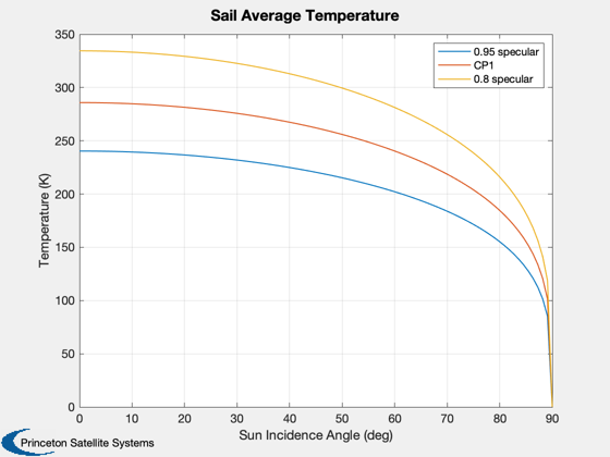
and two other fictional materials. Also computes the temperature, but
note that the temperature is not defined for the perfect sail since it
depends on the absorption coefficient being nonzero.

Since version 7.
------------------------------------------------------------------------
See also SailMesh, CP1Props, SolarPressureForce, PolygonProps, Figui,
Plot2D, Dot, Mag, Unit, SolarFlx
------------------------------------------------------------------------

Contents

%-------------------------------------------------------------------------------
%	 Copyright 2009 Princeton Satellite Systems, Inc.
%-------------------------------------------------------------------------------

% These sails have a nominal front normal of [0;0;1], +Z.

Circular sail perimeter

%------------------------
theta = linspace(0,2*pi,20);
theta = theta(1:end-1);
rSail = 50;  % m
x = rSail*cos(theta);
y = rSail*sin(theta);
[v,f] = SailMesh( x, y );
[a, n, r] = PolygonProps( v, f );
nEl = length(a);

CP1 properties - about 90% specular

%------------------------------------
[optical, infrared, thermal] = CP1Props;
specular = [1 0.95 optical.sigmaS(1) 0.8];
diffuse  = [0 0.01 optical.sigmaD(1) 0.05];
absorp   = [0 0.04 optical.sigmaA(1) 0.15];

Solar flux at 1 AU

%--------------------
flux = SolarFlx( 1.0 );

Create a vector of incidence angles in x/z plane

%-------------------------------------------------
theta = linspace(0,pi/2);
nPts  = length(theta);
uSun  = [sin(theta);zeros(size(theta));cos(theta)];

fTotal = cell(1,4);
coneAngle = zeros(4,nPts);
centerAngle = zeros(4,nPts);
Tavg = zeros(4,nPts);

for k = 1:4

  opt = optical;
  % Assign front properties
  opt.sigmaS(1) = specular(k);
  opt.sigmaD(1) = diffuse(k);
  opt.sigmaA(1) = absorp(k);

  ems = thermal.emissivity;

  fSail = zeros(3,nPts);

  % Compute the force and temperature of each element
  %--------------------------------------------------
  for j = 1:nPts
    [fEl, T, fT] = SolarPressureForce( a', n', uSun(:,j), flux, ...
                                           opt, ems );
    Tavg(k,j) = mean(T);
    fSail(:,j) = fT;
  end

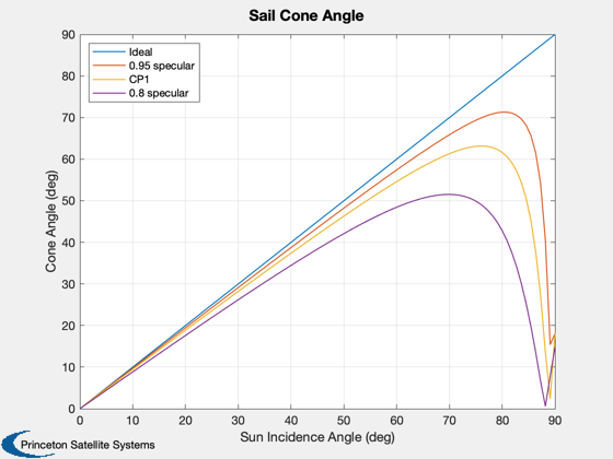
  coneAngle(k,:) = acos(Dot(Unit(fSail),-uSun));
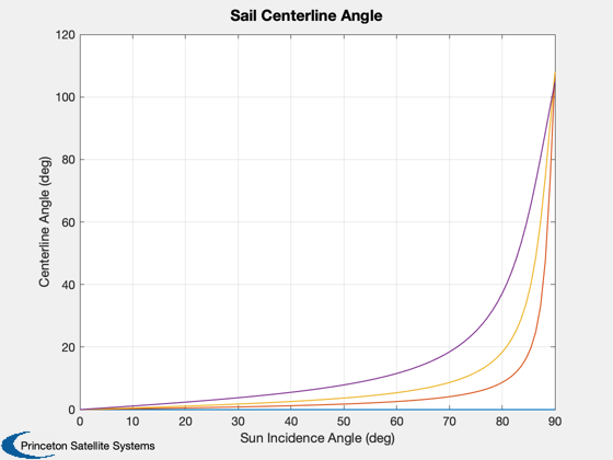
  centerAngle(k,:) = acos(Dot(Unit(fSail),-[0;0;1]));
  fTotal{k} = fSail;

end

Plot the results

%-----------------
% Sail vector performance
angles = theta*180/pi;
aLabl = 'Sun Incidence Angle (deg)';
sailLabl = {'Ideal', '0.95 specular', 'CP1', '0.8 specular'};
Plot2D(angles, [fTotal{1}([1 3],:)]*1000, aLabl,{'Fx','Fz'},'Sail Force Vector (mN)');
subplot(2,1,1)
hold on
plot(angles, fTotal{2}(1,:)*1000, 'g');
plot(angles, fTotal{3}(1,:)*1000, 'r');
plot(angles, fTotal{4}(1,:)*1000, 'c');
subplot(2,1,2)
hold on
plot(angles, fTotal{2}(3,:)*1000, 'g');
plot(angles, fTotal{3}(3,:)*1000, 'r');
plot(angles, fTotal{4}(3,:)*1000, 'c');
legend(sailLabl{:},'location','southeast')

% Force magnitude alone on big plot
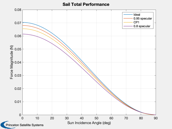
Plot2D(angles, [Mag(fTotal{1});Mag(fTotal{2});Mag(fTotal{3});Mag(fTotal{4})], ...
    aLabl,'Force Magnitude (N)','Sail Total Performance');
legend(sailLabl{:});

% CONE angle
Plot2D(angles, coneAngle*180/pi, aLabl,'Cone Angle (deg)','Sail Cone Angle');
legend(sailLabl{:},'location','NorthWest');

% CENTERLINE angle
Plot2D(angles, centerAngle*180/pi,...
  aLabl,'Centerline Angle (deg)','Sail Centerline Angle');

% Sail material average temperature
Plot2D(angles, Tavg(2:4,:),...
  aLabl,'Temperature (K)','Sail Average Temperature');
legend(sailLabl{2:4});

Figui;

%--------------------------------------
% PSS internal file version information
%--------------------------------------

Published with MATLAB® R2020a