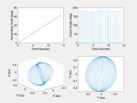
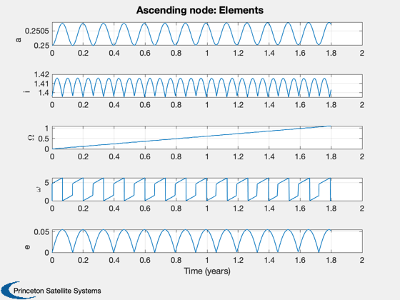
Simulate a heliocentric locally optimal trajectory.
You can simulate any one of four types. You can also change the direction,
i.e. increase or decrease the element in question.
This uses the control laws developed in McInnes and is designed to exactly
duplicate the images in his book, Fig. 4.19, 4.20, 4.22, and 4.24, however
there some inconsistencies between the sail properties listed in the text
and the graphics.
Functions demonstrated:
    ConeClockConvention
    LocallyOptimalTraj
    FSailGuidance
The ascending node and inclination plots also shown the analytical increase
expected in these elements for the given sail acceleration and orbit (red).
Since version 7.
------------------------------------------------------------------------
Reference: Colin R. McInnes, "Solar Sailing: Technology, Dynamics and Mission
           Applications", Springer Praxis, London, 1999, pp. 136-148.
------------------------------------------------------------------------
See also IConv, Constant, InformDlg, NewFig, Plot2D, TimeLabl,
UnwrapPhase, El2RV, M2Nu, Period, RV2El, RVFromKepler,
ConeClockConvention, delta, LocallyOptimalTraj, FSailGuidance
------------------------------------------------------------------------
Contents
%-------------------------------------------------------------------------------
%   Copyright (c) 2005 Princeton Satellite Systems, Inc.
%   All rights reserved.
%-------------------------------------------------------------------------------

clear d;
USER PARAMETERS:
Possible control type examples
%-------------------------------
% 1. ascending node
% 2. eccentricity
% 3. inclination
% 4. semi-major axis
% 5. Your custom elements and control (edit case below)
kControlType = 1;
% Direction flag: +/- 1
%----------------------
direction = 1;
% Cone/Clock convention
%----------------------
% 1. Cone angle kept positive
% 2. Clock angle kept to [0,pi)
iConv = 2;
%%%%%%%%%%%%%%%%%%%%%%%%%
Set up the parameters
%----------------------
d.mu          = Constant('mu sun');
a             = 0.3*1e-6; % 0.3 mm/s^2 converted to km/s^2
beta          = 0.05;
Initial conditions
%-------------------
au = Constant('au');
switch kControlType
  case 1
    % Demonstrate ascending node change
    x0            = au/4;                    % start at 0.25 AU
    el0           = [x0;80*pi/180;0;0;0;0];  % 80 deg inclination
    nYears        = 1.8;                     % 1.8 years
    dEl           = 88.2/sin(el0(2))*beta;   % analytical change
  case 2
    % Demonstrate eccentricity change
    x0            = 1.25*au;
    el0           = [x0;0;0;0;0.2;0];
    nYears        = 6.67; %7.07 unconstrained, 6.65 constrained
    if (direction < 0)
      nYears = 3;
    end
  case 3
    % Demonstrate inclination change
    x0            = au/4;
    el0           = [x0;0;0;pi/2;0;0];
    nYears        = 1;
    if (direction < 0)
      el0(2) = 1.4;
    end
    dEl           = 88.2*beta;
  case 4
    % Demonstrate semi-major axis change
    x0            = 1.25*au;
    el0           = [x0;0;0;0;0.2;0];
    nYears        = 8.8;
    if (direction < 0)
      nYears = 2;
    end
  otherwise
    % Your custom elements and control selection
    x0      = 1.25*au;
    el0     = [x0;0.5;0;0;0.2;0];
    nYears  = 1;
    kControlType = 4;

end
[r0,v0]       = El2RV( el0, [], d.mu );
x             = [r0;v0];
Control details
%----------------
controlTypes = {'ascending node','eccentricity','inclination','semi-major axis','custom'};
controlType  = controlTypes{kControlType};
disp(' ')
disp('LocalOptimalSim.')
disp(['Control type selected: ' controlType])
disp(['Direction: ' num2str(direction)])
LocalOptimalSim.
Control type selected: ascending node
Direction: 1
Integrate the trajectory
%-------------------------
hDlg = InformDlg( 'Integrating...', 'LocalOptimalMission' );
odeOptions = odeset('AbsTol',1e-6,'RelTol',1e-5);
[t,z] = ode113( @FSailGuidance, [0 nYears*365.25*86400], x, odeOptions,...
                 a, [], [], d.mu, struct('type',controlType,'dirFlag',direction) );
nSim = length(t);
close(hDlg);
Plotting array
%---------------
el     = zeros(6,nSim);
angles = zeros(2,nSim);
nu     = zeros(1,nSim);

tPlot = t';
xPlot = z';
Process the orbital elements
%-----------------------------
r = z(:,1:3)';
v = z(:,4:6)';
for k = 1:nSim
  el(:,k) = RV2El( r(:,k), v(:,k), d.mu )';
  [alpha, delta] = LocallyOptimalTraj( controlType, r(:,k), v(:,k), d.mu, direction );
  angles(:,k) = [alpha;delta];
  nu(k)       = M2Nu(el(5,k),el(6,k));
end
disp('Finished.')
Finished.
Plot the results
%-----------------
[t, tL] = TimeLabl( tPlot );
controlType(1) = upper(controlType(1));
orbNum = tPlot/Period(x0,d.mu);
[alpha,delta] = ConeClockConvention(angles(1,:),angles(2,:),iConv);

switch kControlType
  case {4,2}
    orbNum = UnwrapPhase(nu)/(2*pi);

    % Semi-major axis and eccentricity
    [rI,vI] = RVFromKepler(el0,[],d.mu);
    NewFig([controlType ': Orbit and Cone Angle']);
    subplot(2,2,1);
    plot(orbNum,el(1,:)/au);
    ylabel('Semi-major axis (au)'); xlabel('Orbit Number')
    grid on
    subplot(2,2,2);
    plot(orbNum,el(5,:));
    ylabel('Eccentricity'); xlabel('Orbit Number')
    grid on
    subplot(2,2,3);
    plot(orbNum,angles(1,:)*180/pi);
    ylabel('Pitch angle (deg)'); xlabel('Orbit Number')
    subplot(2,2,4);
    plot(xPlot(1,:)/au, xPlot(2,:)/au);
    hold on
    plot(rI(1,:)/au, rI(2,:)/au, '--');
    xlabel('x (au)'); ylabel('y (au)')
    axis equal

    Plot2D(orbNum,[alpha;delta],'Orbit Number',{'\alpha' '\delta'},[controlType ': Angles'])
  case {1,3}
    % Analytical increase (deg/orbit)
    del = dEl*orbNum;
    NewFig([controlType ': Orbit and Clock Angle']);
    elk = [3 0 2];
    lbl = {'Ascending Node (deg)' ' ' 'Inclination (deg)'};
    subplot(2,2,1);
    plot(orbNum,el(elk(kControlType),:)*180/pi);
    hold on; plot(orbNum,del,'r');
    ylabel(lbl{kControlType}); xlabel('Orbit Number')
    grid on
    subplot(2,2,2);
    [alpha2,delta2] = ConeClockConvention(angles(1,:),angles(2,:),1);
    plot(orbNum,delta2*180/pi);
    ylabel('Clock Angle (deg)'); xlabel('Orbit Number')
    grid on
    subplot(2,2,3);
    plot3(xPlot(1,:)/au,xPlot(2,:)/au,xPlot(3,:)/au);
    xlabel('X (au)'); ylabel('Y (au)'); zlabel('Z (au)');
    grid on
    subplot(2,2,4);
    plot(xPlot(2,:)/au, xPlot(3,:)/au);
    xlabel('Y (au)'); ylabel('Z (au)');
    grid on
    axis equal

    Plot2D(t,[el(1,:)/au;el(2:5,:)],tL,{'a' 'i' '\Omega' '\omega' 'e'},[controlType ': Elements'])


end


%--------------------------------------
% PSS internal file version information
%--------------------------------------