Fly near an invariant parabolic manifold and control to the displaced orbit.

This is a possible transfer for an Earth magnetotail science mission. The optimal orbit rate is used for the displaced orbit.

Since version 7.
------------------------------------------------------------------------
Reference: John Bookless and Colin McInnes, "Dynamics and Control of
Displaced Periodic Orbits Using Solar-Sail Propulsion", JOURNAL OF
GUIDANCE, CONTROL, AND DYNAMICS, Vol. 29, No. 3, May-June 2006
------------------------------------------------------------------------
See also NonKeplerianPlanet and SailClosedLoopNLEqns., QCR, Constant,
Plot2D, Plot3D, TimeLabl, PlottingTool, PlottingToolStruct, Accel,
PlottingParabolas, Control
------------------------------------------------------------------------

Contents

%---------------------------------------------------------------------------
%   Copyright (c) 2007 Princeton Satellite Systems, Inc.
%   All rights reserved.
%--------------------------------------------------------------------------

Desired Orbit Parameters

%-------------------------
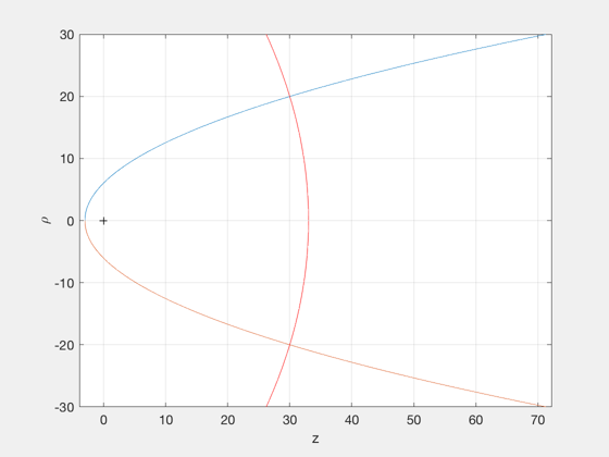
rho0 = 20;
z0   = 30;
PlottingParabolas( rho0, z0 );

Simulation duration (non-dimensional)

%--------------------------------------
tEnd = 6e3;

Control mode: (0) none (1) sail area (2) sail pitch angle

%----------------------------------------------------------
mode = 1;

Dimensionless

%--------------
mu = 1;

Compute orbit parameters

%---------------------------
r0 = (rho0^2 + z0^2)^(1/2);
thetadot0 = (rho0^2 + z0^2)^(-3/4);
hz0 = rho0^2*thetadot0;
% Assume optimal period
kappa0 = z0/r0^3;  % non-dimensional
% Compute angular momentum of desired orbit
H = 0.5*(rho0^2*thetadot0^2) - mu/r0 - kappa0*z0;
xi0 = sqrt(z0+r0);
eta0 = sqrt(r0-z0);

Compute manifold insertion conditions

%--------------------------------------
zin = 0;
rin = eta0^2;
rhoin = rin;
thetadotin = hz0/rhoin^2;
rhodotin = sqrt(H + mu/rin + kappa0*zin - 0.5*rhoin^2*thetadotin^2);
zdotin = rhodotin;

Design Linear Controller

%-------------------------
A31 = -3*hz0^2/rho0^4 - 1/r0^3 +3*rho0^2/r0^5;
A32 = 3*rho0*z0/r0^5;
A41 = A32;
A42 = -1/r0^3 + 3*z0^2/r0^5;
A = [0 0 1 0;0 0 0 1; A31 A32 0 0;A41 A42 0 0];

switch mode
  case 1
    % Sail area control
    B = [0;0;0;1];
    Q = diag([1e-2 1e-2 1e-2 1e-2]);
    R = 1e6;
  case 2
    % Pitch angle control
    B = [0;0;kappa0;0];
    Q = diag([1e1 1e1 1e-1 1e-1]);
    R = 1e4;
end
N = [0;0;0;0];
[G,sinf] = QCR(A,B,Q,R,N);

Set up and perform integration

%-------------------------------
tspan = [0 tEnd];
xin = [rhoin zin rhodotin zdotin 0 thetadotin]';
options = odeset('RelTol',1e-10,'AbsTol',1e-12);
[t,x] = ode45(@SailClosedLoopNLEqns,tspan,xin,options,kappa0,rho0,z0,G,mode);

Plot Results

%-------------
n = length(t);
PxiP = zeros(1,n);
PetaP = zeros(1,n);
control = 0;

Compute cartesian coords from cylindrical

%------------------------------------------
xP = x(:,1)'.*sin(x(:,5)');
yP = x(:,1)'.*cos(x(:,5)');
zP = x(:,2)';
rP = sqrt(x(:,1)'.^2+x(:,2)'.^2);
xi = sqrt(rP+zP);
eta = sqrt(rP-zP);

Compute parabolic quantities

%------------------------------
for i = 1:n
    xidot = (1/(2*xi(i)))*(x(i,4) + (1/rP(i))*(x(i,4)+x(i,3)));
    etadot = (1/(2*eta(i)))*(-x(i,4) + (1/rP(i))*(x(i,4)+x(i,3)));
    PxiP(i) = xidot*(xi(i)^2+eta(i)^2);
    PetaP(i) = etadot*(xi(i)^2+eta(i)^2);
end

Dimensionalize for the Earth

%-----------------------------
muEarth = Constant('mu earth');
rE      = 6378;
wTilde = sqrt(muEarth/rE^3);
kTilde = muEarth/rE^2;
[tPlot,tLabl] = TimeLabl(t'*1/wTilde);

Sail size

%----------
[pitch,accel] = NonKeplerianPlanet( rho0*6378, z0*6378, [], Constant('mu earth') );
fprintf('Sail accel: %5.5f mm/s2\n',accel*1e6)

Sail accel: 6.27155 mm/s2

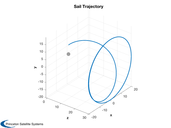
Plot trajectory and coordinates

%--------------------------------
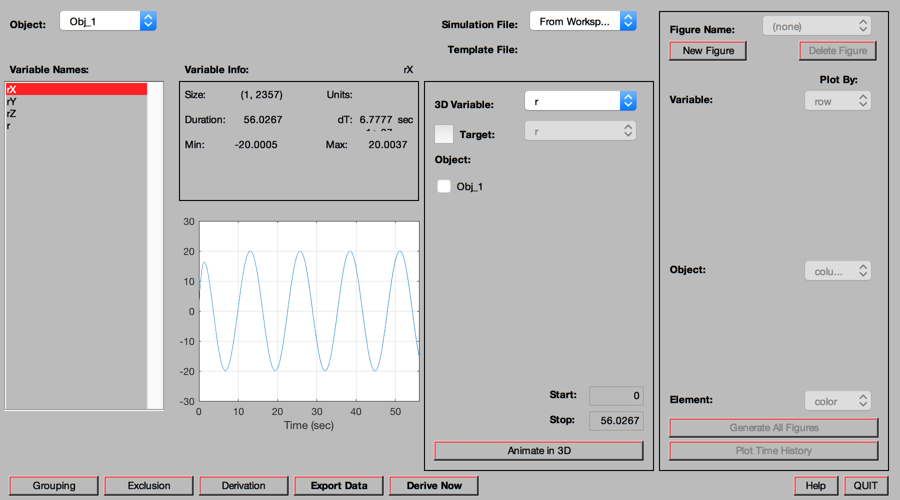
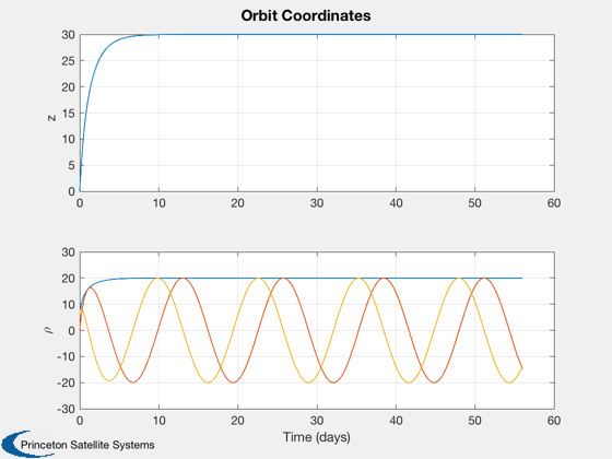
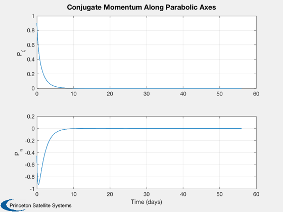
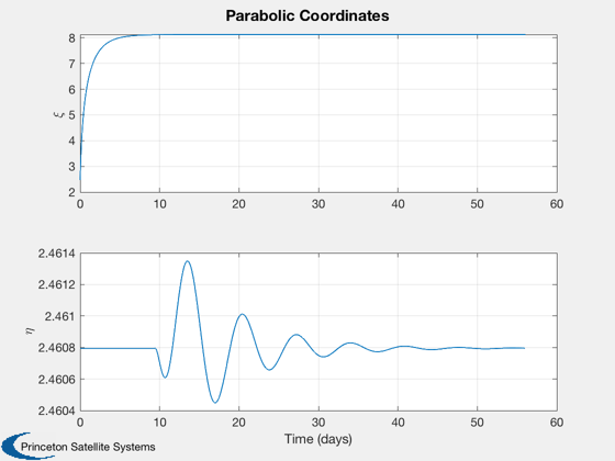
Plot3D([zP;xP;yP],'z','x','y','Sail Trajectory',1)
Plot2D(tPlot,[zP;x(:,1)';xP;yP],tLabl,{'z','\rho'},'Orbit Coordinates',[],...
  {[1],[2 3 4]})
Plot2D(tPlot,[PxiP;PetaP],tLabl,{'P_{\xi}','P_{\eta}'},'Conjugate Momentum Along Parabolic Axes')
Plot2D(tPlot,[xi;eta],tLabl,{'\xi','\eta'},'Parabolic Coordinates')

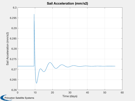
Computing Control

%------------------
kappaP = kappa0*ones(1,n);
alphaP = zeros(1,n);
for i=1:n
    if abs(x(i,1)-rho0) <= .02
      control = -(G(1)*(x(i,1)-rho0) + G(2)*(x(i,2)-z0) + G(3)*x(i,3) + G(4)*x(i,4));
      kappaP(i) = kappa0 + control;
      alphaP(i) = control;
    end
end
switch mode
  case 1
    Plot2D(tPlot,kappaP*kTilde*1e6,tLabl,'Sail Acceleration (mm/s2)')
  case 2
    psiP = asin(sin(alphaP).*cos(x(:,5)'));
    phiP = atan(tan(alphaP).*sin(x(:,5)'));
    Plot2D(tPlot,[psiP;phiP]*180/pi,tLabl,{'Pitch','Yaw'},'Sail Control Angles (degrees)')
end

d = PlottingToolStruct( [xP;yP;zP], tPlot );
PlottingTool( 'load sim data', d );


%--------------------------------------
% PSS internal file version information
%--------------------------------------

Published with MATLAB® R2019a