Solar Polar Imager demo with JPL optimal trajectory data.

Verify clock conversions by comparing against McInnes format. Simple Sun gravity model suffices.

------------------------------------------------------------------------
See also FSailJPL and FSailGuidance., Cone, Constant, Plot2D, Plot3D,
Cross, Mag, RK45, Unit, PlotOrbitPage, El2RV, Nu2M, RV2El,
ClockConversion, delta, LocallyOptimalTraj
------------------------------------------------------------------------

Contents

%-------------------------------------------------------------------------------
%	  Copyright (c) 2005,2006 Princeton Satellite Systems, Inc.
%   All rights reserved.
%   Since version 7.
%-------------------------------------------------------------------------------

%%%%%%%%%%%%%%%%%%%%%%%%%%%%%%%%%%%%%%%%%%%%%%%%%%%%%%%%%
% User Parameters
phase = 1;       % Phase 1, points to 440. Phase 2, beyond.
integration = 2; % 1, JPL angles. 2, McInnes conversion.
plotHistory = 0; % 1, plot full trajectory. 0, don't.
%%%%%%%%%%%%%%%%%%%%%%%%%%%%%%%%%%%%%%%%%%%%%%%%%%%%%%%%%

d = load('SPIData.mat');

deg2rad = pi/180;
muSun   = 132712440017.987;
au      = Constant('au');

Use only nonzero angle data points (from inspection)

%-----------------------------------------------------
nPts = 1292;
jD   = d.data(2:(nPts+1),2)'+2450000.0;
days = d.data(2:(nPts+1),1)';
% Elements are stored in AU and degrees
elJPL = d.data(2:(nPts+1),20+[1:6])';
cone  = d.data(2:(nPts+1),9)';
clock = d.data(2:(nPts+1),10)';
acc   = d.data(2:(nPts+1),12)';

% Convert elements to km and radians and reorder
% PSS format: [a;i;W;w;e;M]

JPL order: [a;e;i;W;w;f]

%------------------------------------------------
el      = zeros(size(elJPL));
el(1,:) = elJPL(1,1:nPts)*au;               % sma
el(2,:) = elJPL(3,1:nPts)*pi/180;           % inc
el(3,:) = elJPL(4,1:nPts)*pi/180;           % lan
el(4,:) = elJPL(5,1:nPts)*pi/180;           % apf
el(5,:) = elJPL(2,1:nPts);                  % ecc
el(6,:) = Nu2M( el(5,:), elJPL(6,:)*pi/180 ); % M
[r,v]   = El2RV( el, [], muSun );

% Last elements of JPL output reversed???
% Mean anomaly and |r| of last portion constant.
el(4,:) = elJPL(6,1:nPts)*pi/180;           % apf
el(6,:) = Nu2M( el(5,:), elJPL(5,:)*pi/180 ); % M
[r,v]   = El2RV( el, [], muSun );

if plotHistory
  % Plot trajectory data for confirmation
  %--------------------------------------
  PlotOrbitPage(r/au,days(1:nPts),'SPI Trajectory (JPL)')
  Plot2D(days,[cone;clock],'Time (days)',{'Cone','Clock'},'SPI Angles (JPL)')
  Plot2D(days,el([1 2 5],:),'Time',{'SMA','Inc','Ecc'})
end

Convert clock to McInnes format

%--------------------------------
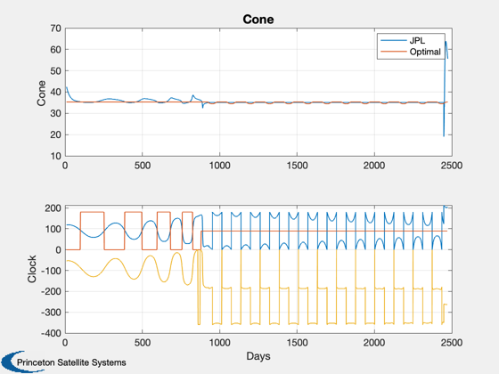
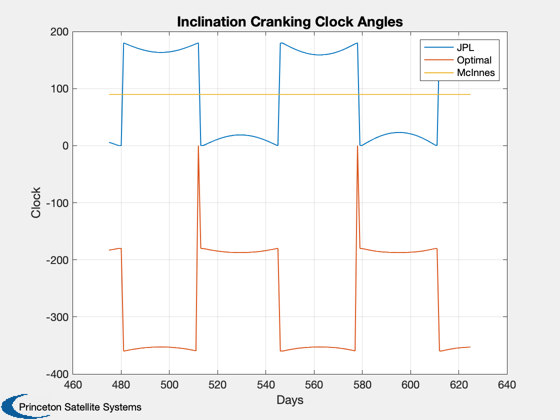
clockNew = zeros(1,nPts);
alpha = zeros(1,nPts);
delta = zeros(1,nPts);
dCC = struct('r',r,'v',v,'s',-Unit(r),'eciFlag',0);
clockNew = ClockConversion( cone*deg2rad, clock*deg2rad, 3, 1, dCC )/deg2rad;
% Compare to locally optimal law (McInnes)
[alpha1, delta1] = LocallyOptimalTraj( 'inclination', r(:,6:440), v(:,6:440), muSun, 1 );
alpha(6:440) = alpha1;
delta(6:440) = delta1;

[alpha2, delta2] = LocallyOptimalTraj( 'semi-major axis', r(:,441:end), v(:,441:end), muSun, 1 );
alpha(441:end) = alpha2;
delta(441:end) = delta2;
Plot2D(days(6:nPts),[cone(6:nPts);clock(6:end);-clockNew(6:end);alpha(6:end)/deg2rad;delta(6:end)/deg2rad],...
  'Days',{'Cone','Clock'},'','lin',{'[1 4]','[2 5 3]'})
legend('JPL','Optimal','McInnes')
% Zoom in on cranking
nSelect = 475:625;
Plot2D(nSelect,[clock(nSelect);-clockNew(nSelect);delta(nSelect)/deg2rad],...
  'Days',{'Clock'},'Inclination Cranking Clock Angles')
legend('JPL','Optimal','McInnes')

% Try integrating with sail angles

Warning: Ignoring extra legend entries. 

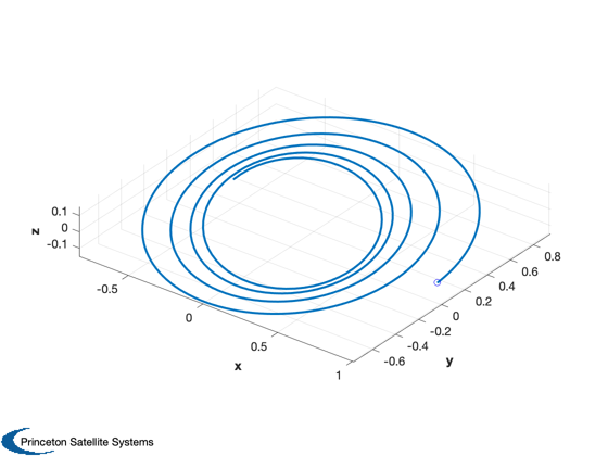
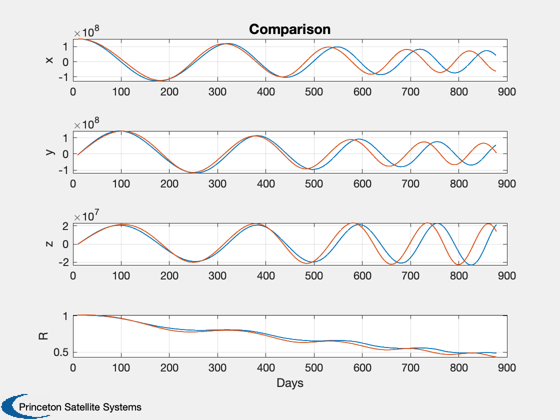
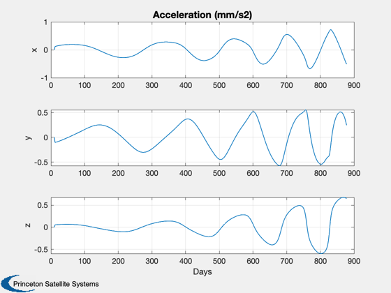
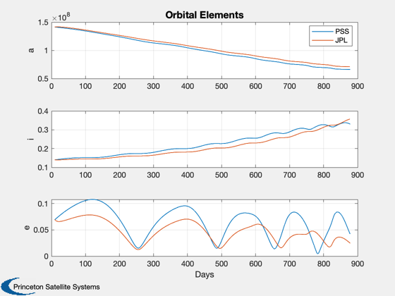
semi-major axis change: to point 440

%-----------------------------------------------
switch phase
  case 1
    nMin = 6;
    nMax = 440;
  case 2
    nMin = 450;
    nMax = 650;
end
x = [r(:,nMin); v(:,nMin)];
xPlot = zeros(6,nMax-nMin+1);
aPlot = zeros(3,nMax-nMin+1);
elPlot = zeros(6,nMax-nMin+1);
xPlot(:,1) = x;
elPlot(:,1) = RV2El(x(1:3),x(4:6),muSun);
muSun = Constant('mu sun');
kP = 2;
coneR = cone*deg2rad;
clockR = clock*deg2rad;
% characteristic acceleration
a0     = acc(6)*Mag(r(:,6))^2/au^2/cos(cone(6)*pi/180)^2*1e-6;
for k = (nMin):(nMax-1)
  cC = cos(coneR(k));
  sC = sin(coneR(k));
  cL = cos(clockR(k));
  sL = sin(clockR(k));
  % heliocentric clock frame - sail normal
  xHat = -Unit(x(1:3));
  zHat = Unit(Cross(xHat,[0;0;1]));
  yHat = Unit(Cross(zHat,xHat)); % Projection of North ecliptic
  nSail = cC*xHat + sC*cL*yHat + sC*sL*zHat;

  dT = (days(k+1)-days(k))*86400;
  if dT~=0
    switch integration
      case 1
        [x,hLast] = RK45( 'FSailJPL', x, dT, dT, 8640, 1e-8, days(k), acc(k)*1e-6, coneR(k), clockR(k), muSun );
      case 2
        %[x,hLast] = RK45( 'FSailGuidance', x, dT, dT, 8640, 1e-6, 0, acc(k)*1e-6/cC^2, coneR(k), -clockNew(k)*deg2rad, muSun );
        [x,hLast] = RK45( 'FSailGuidance', x, dT, dT, 8640, 1e-6, 0, a0, coneR(k), -clockNew(k)*deg2rad, muSun );
    end
  end
  xPlot(:,kP) = x;
  aPlot(:,kP) = -acc(k)*nSail;
  elPlot(:,kP) = RV2El(x(1:3),x(4:6),muSun);
  kP = kP+1;
end
Plot3D(xPlot(1:3,:)/au)
hold on
plot3(xPlot(1,1)/au,xPlot(2,1)/au,xPlot(3,1)/au,'bo')
Plot2D(days(nMin:nMax),[r(1:3,nMin:nMax);xPlot(1:3,:);Mag(r(1:3,nMin:nMax))/au;Mag(xPlot(1:3,:))/au],...
  'Days',{'x','y','z','R'},'Comparison','lin',{[1 4],[2 5],[3 6],[7 8]})
Plot2D(days(nMin:nMax),aPlot,'Days',{'x','y','z'},'Acceleration (mm/s2)')
Plot2D(days(nMin:nMax),[elPlot([1 2 5],:);el([1 2 5],nMin:nMax)],'Days',{'a','i','e'},'Orbital Elements',[],...
  {[1 4],[2 5],[3 6]})
legend('PSS','JPL')


%--------------------------------------
% PSS internal file version information
%--------------------------------------

Published with MATLAB® R2021a