Orbit propagation test.
Propagates orbits in both equinoctial and cartesian coordinates under the influence of a small radial step acceleration. The results are compared with an analytical solution.
Since version 7.
------------------------------------------------------------------------
See also Constant, InformDlg, Plot2D, Mag, El2RV, Accel, ElToMEq,
MEqToRV, RHSCartesianRadialAccel, RHSEquinoctial
------------------------------------------------------------------------
Contents
- Useful constants
- This assumes 100 kg mass, 1x1 m specular sail
- Heliocentric system
- Keplerian elements
- Initial orbit at 1 au in equinoctial
- In cartesian
- End time is 4 years
- Acceleration vector
- Integration (ode113) parameters
- Equinoctial, then in cartesian
- Transpose for plotting
- Plot the equinoctial elements
- Convert equinoctial to cartesian
- Compute the analytical solutions
- Convert into the Hill's frame
- Plot
%-------------------------------------------------------------------------------
%	Copyright (c) 2005-2006 Princeton Satellite Systems, Inc.
%   All rights reserved.
%-------------------------------------------------------------------------------
Useful constants
%-----------------
aU                 = Constant('au');
c                  = Constant('speed of light');
This assumes 100 kg mass, 1x1 m specular sail
%----------------------------------------------
r0                 = aU;
accel              = 2*1367*aU^2*1e-6/(c*100)/r0^2; % km/sec^2
Heliocentric system
%---------------------
d.mu               = Constant('mu sun');
Keplerian elements
%-------------------
el                 = [aU;0;0;0;0;0];
Initial orbit at 1 au in equinoctial
%-------------------------------------
x                  = ElToMEq( el, d.mu );
In cartesian
%-------------
[r, v]             = El2RV( el, [], d.mu );
xC                 = [r;v];
End time is 4 years
%--------------------
tEnd               = 4*365.25*86400; % (s)
Acceleration vector
%--------------------
d.f                = [accel;0;0];
Integration (ode113) parameters
%--------------------------------
oDEOptions         = odeset( 'abstol', 1e-12, 'reltol', 1e-12 );
Equinoctial, then in cartesian
%-------------------------------
hDlg = InformDlg( 'Integrating...', 'PropagationDemo' );
[t, x]             = ode113(@RHSEquinoctial,            [0, tEnd], x,  oDEOptions, d );
[tC, xC]           = ode113(@RHSCartesianRadialAccel,   [0, tEnd], xC, oDEOptions, d );
close(hDlg);
Transpose for plotting
%-----------------------
x                  = x';
t                  = t';
tC                 = tC';
xC                 = xC';
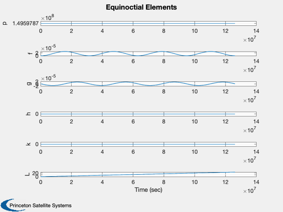
Plot the equinoctial elements
%------------------------------
Plot2D( t, x, 'Time (sec)', {'p' 'f' 'g' 'h' 'k' 'L' }, 'Equinoctial Elements')
Convert equinoctial to cartesian
%---------------------------------
[r, v]             = MEqToRV( x, d.mu );
Compute the analytical solutions
%---------------------------------
r0                 = Mag(r(:,1));
omega              = Mag(v(:,1)/r0);

wt                 = omega*t;
xNom               = accel*[1-cos(wt);-2*(wt - sin(wt))]/omega^2;

wt                 = omega*tC;
xNomC              = accel*[1-cos(wt);-2*(wt - sin(wt))]/omega^2;
Convert into the Hill's frame
%------------------------------
x(1,:)             = Mag(r(1:2,:)) - r0;
x(2,:)             = r0*(unwrap(atan2(r(2,:), r(1,:) )) - omega*t);

clear y
y(1,:)             = Mag(xC(1:2,:)) - r0;
y(2,:)             = r0*(unwrap(atan2(xC(2,:), xC(1,:) )) - omega*tC);
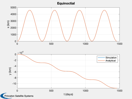
Plot
%-----
Plot2D( t/86400, [x(1:2,:);xNom], 't (days)', {'x (km)' 'y (km)'},'Equinoctial','lin',{'[1 3]' '[2 4]'} );
legend('Simulation','Analytical')

Plot2D( tC/86400, [y(1:2,:);xNomC], 't (days)', {'x (km)' 'y (km)'},'Cartesian','lin',{'[1 3]' '[2 4]'} );
legend('Simulation','Analytical')


%--------------------------------------
% PSS internal file version information
%--------------------------------------