UKF/UKS demonstration.

This is for a 1 dimensional launch problem with an angle sensor that
measures the angle to the launch vehicle. The vehicle is subject
to Gaussian random thrust variations. The sensor is subject to Gaussian
white noise.

The script first runs the simulation and the sensor angle are used
for both the forward and backward Unscented Kalman filters.

The geometry gets worse as the launch vehicle gets higher.

The demo uses UKFUpdate and UKFPredict which are alternatives to UKF.

Since version 11.

%--------------------------------------------------------------------------
%  See also RHSX, AngleSensor, KFInitialize, UKFWeight, UKFPredict,
%  UKFUpdate, KalmanFilterCombine
%--------------------------------------------------------------------------

%--------------------------------------------------------------------------
%   Copyright (c) 2012 Princeton Satellite Systems, Inc.
%   All rights reserved.
%--------------------------------------------------------------------------

clear u pP d

n               = 800;
dT              = 1;

sigmaT          = 0.01;
sigmaTheta      = 0.01;

d               = struct;
d.m             = 1;
d.t0            = 11;
d.g             = 9.806;
d.b             = 1000;
d.tNoise        = sigmaT;
d.noise   	    = sigmaTheta;

% Run the simulation
%-------------------
x     = [0;0];
theta = 0;
t     = 0;
xS    = zeros(3,n);
for k = 1:n

    % Measurement
    %------------
    theta       = AngleSensor(x,d);

	  % State update
    %-------------
    x           = RK4( 'RHSX', x, dT, 0, d );

    % Store for plotting and processing in the UKS
    %---------------------------------------------
    xS(:,k)     = [x;theta];
end

% Estimation parameters
%----------------------
dUKF          = d;

% Initialize the Kalman Filter
%-----------------------------
u      = KFInitialize( 'ukf','f',@RHSX,'alpha',1,...
                        'kappa',length(x)-2,'beta',2,'dT',dT,'fData',dUKF,...
                        'p',diag([0.1 0.01]),'q',diag([0 sigmaT^2]),'x',x, 'm',x);

% Get the UKF weights
%--------------------
u = UKFWeight( u );

% UKF without measurements which is just the prediction step
%-----------------------------------------------------------
t = 0;

pP = cell(n);
xF = zeros(4,n);

for k = 1:n
  % Store for plotting
  %------------------
  xF(:,k)	= [u.m;diag(u.p)];
  pP{k}	= u.p;

  % UKF
  %----
  u.t 	= t;
  u       = UKFPredict( u );
  t       = t + dT;
end


xB0 = u.m;
pB0 = u.p;

[t,tL] = TimeLabl((0:(n-1))*dT);

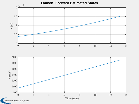
Plot2D(t,xF(1:2,:),tL,{'x (m)' 'v (m/s)' },'Launch: Forward Estimated States')
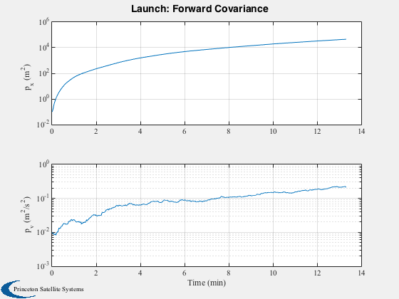
Plot2D(t,xF(3:4,:),tL,{'p_x (m^2)' 'p_v (m^2/s^2)'},'Launch: Forward Covariance','ylog')

u.p = diag([0.1 0.01]);
u.m = [0;0];

% UKF
%----
t  = 0;
pF = cell(n);
for k = 1:n
  % Store for plotting
  %------------------
  xF(:,k)         = [u.m;diag(u.p)];
  pF{k}           = u.p;

  % UKF
  %----
  u.t             = t;
  u.y.data        = xS(3,k);
  u.y.param.hFun	= @AngleSensor;
  u.y.param.hData	= dUKF;
  u.y.param.r 	= sigmaTheta^2;
  u               = UKFPredict( u );
  u               = UKFUpdate( u );
  t               = t + dT;
end


% UKS
%----

% Flip the sign of the time step
%-------------------------------
u.dT            = -dT;
u.p             = pB0;
u.m             = xB0;
t               = t(end);

pB              = cell(n);
xB              = zeros(4,n);
for k = n:-1:1

  % Store for plotting
  %-------------------
  xB(:,k)         = [u.m;diag(u.p)];
  pB{k}           = u.p;

  % UKF
  %----
  u.t             = t;
  u.y.data        = xS(3,k);
  u.y.param.hFun	= @AngleSensor;
  u.y.param.hData	= dUKF;
  u.y.param.r 	= sigmaTheta^2;
  u               = UKFPredict( u );
  u               = UKFUpdate( u );

  t               = t - dT;

end

xC = zeros(4,n);

for k = 1:n
    [xS, pS] = KalmanFilterCombine( xB(1:2,k), pB{k}, xF(1:2,k), pF{k} );
    xC(:,k)  = [xS;diag(pS)];
end

[t,tL] = TimeLabl((0:(n-1))*dT);

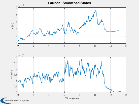
Plot2D(t,xC(1:2,:),                  tL, {'x (m)' 'v (m/s)'},          'Launch: Smoothed States')
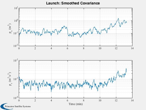
Plot2D(t,xC(3:4,:),                  tL, {'p_x (m^2)' 'p_v (m^2/s^2)'},'Launch: Smoothed Covariance','ylog')
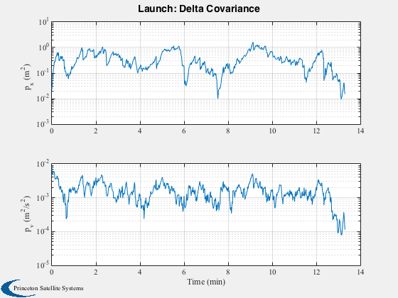
Plot2D(t,abs(xC(3:4,:) - xF(3:4,:)), tL, {'p_x (m^2)' 'p_v (m^2/s^2)'},'Launch: Delta Covariance',   'ylog')


%--------------------------------------
% PSS internal file version information
%--------------------------------------