Contents

Demo of the mimimum time and maximum distance straight-line functions.

For a given set of engine parameters, there are limits to what can be achieved for a straight-line mission, which is defined by a distance and a time to get there. This is a comprehensive set of demos of the straight-line functions.

------------------------------------------------------------------------
See also: ZeroPayloadDistance, ZeroPayloadTime, ComputeThrust,
ComputePayloadFraction, EnginePower
------------------------------------------------------------------------

%--------------------------------------------------------------------------
%	Copyright (c) 2018 Princeton Satellite Systems, Inc.
%   All rights reserved.
%--------------------------------------------------------------------------

Engine and mission parameters

specific power, W/kg

sigma = 1000;
% structural fraction, kg tank/kg fuel
f     = 0.05;
% thrust efficiency
eta   = 0.4;
% exhaust velocity (km/s)
uE0 = 100;

au = Constant('au');
year = 365.25*86400;

uEs = [75 150 300];
tFs = linspace(0,10,101);
d0s = linspace(1,125,125);

d = Straight2DStructure;
d.eta = eta;
d.f = f;
d.sigma = sigma;
d.tF = year;
d.dF = 5*au;
d.mP = 100;

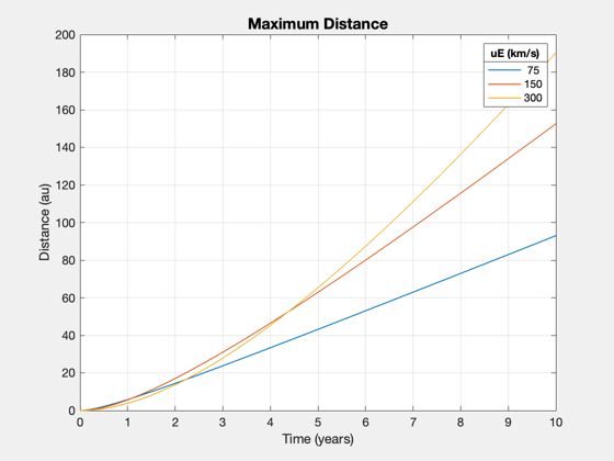
Maximum distance from a fixed time

dMax = [];
for k = 1:length(uEs)
  dMax(k,:) = ZeroPayloadDistance( tFs*year, uEs(k), sigma, eta, f );
end
Plot2D(tFs,dMax/au,'Time (years)','Distance (au)','Maximum Distance');
ll = legend(num2str(uEs'));
ll.Title.String = 'uE (km/s)';

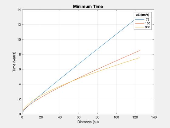
Minimum time for a fixed distance

tFv = zeros(length(uEs),length(d0s));
for k = 1:length(uEs)
  tFv(k,:) = ZeroPayloadTime( d0s*au, uEs(k), sigma, eta, f );
end
Plot2D(d0s,tFv/year,'Distance (au)','Time (years)','Minimum Time');
ll = legend(num2str(uEs'));
ll.Title.String = 'uE (km/s)';

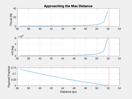
Select a time and make plots for payload

d.tF = 5*year;
d.uE = uE0;
dM = ZeroPayloadDistance( d );
dFs = linspace(0.7,0.995,25)*dM;
thrust = zeros(1,length(dFs));
m0 = zeros(1,length(dFs));
for k = 1:length(dFs)
  d.dF = dFs(k);
  thrust(k) = ComputeThrust( d );
  m0(k) = InitialMass( thrust(k), d );
end
Plot2D(dFs/au,[thrust;m0;d.mP./m0],'Distance (au)',{'Thrust (N)','m0 (kg)','Payload Fraction'},'Approaching the Max Distance')
subplot(3,1,1)
hold on;
yy = axis;
plot(dM/au*[1 1],yy(3:4),'r-')
subplot(3,1,2)
hold on;
yy = axis;
plot(dM/au*[1 1],yy(3:4),'r-')
subplot(3,1,3)
hold on;
yy = axis;
plot(dM/au*[1 1],yy(3:4),'r-')

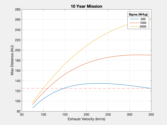
Mission with exhaust velocity

uEv = linspace(75,350,50);
tF  = 10*year;
dUe = [];
sigmas = [500 1000 2000];
for j = 1:3
  for k = 1:length(uEv)
    dUe(j,k) = ZeroPayloadDistance( tF, uEv(k), sigmas(j), eta, f );
  end
end
Plot2D(uEv,dUe/au,'Exhaust Velocity (km/s)','Max Distance (AU)','10 Year Mission')
hold on;
yy = axis;
plot(yy(1:2),125*[1 1],'r--')
ll = legend(num2str(sigmas'));
ll.Title.String = 'Sigma (W/kg)';

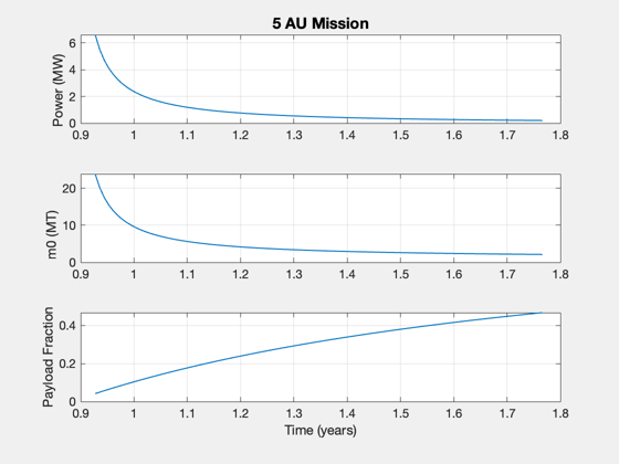
Select a distance and make plots

dF = 5*au;  % Jupiter mission
sigma = 1000;
tMin = ZeroPayloadTime( dF, uE0, sigma, eta, f );
tVec = linspace(1.05*tMin,2*tMin);
d.dF = dF;
d.mP = 1000;
m0 = [];
thrust = [];
lambda = [];
alpha = [];
m0 = [];
for k = 1:length(tVec)
  d.tF = tVec(k);
  [lambda(k),alpha(k)] = ComputePayloadFraction( d );
  thrust(k) = ComputeThrust( d );
  m0(k) = InitialMass( thrust(k), d );
end
powers = EnginePower( thrust, d );
Plot2D(tVec/year,[powers*1e-6;m0*1e-3;d.mP./m0],'Time (years)',{'Power (MW)','m0 (MT)','Payload Fraction'},'5 AU Mission')
%gtext('Payload mass: 1000 kg')

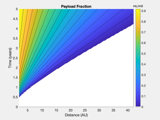
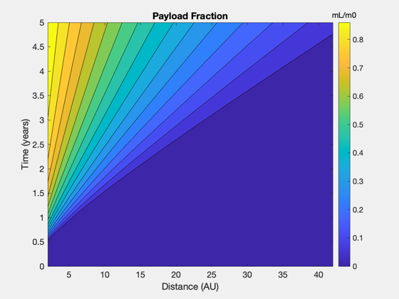
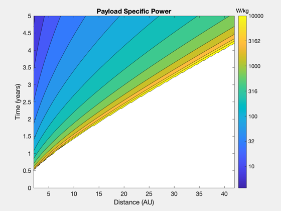
Distance and time surfaces - payload fraction and specific power

Planetary system - to 40 AU

uE = uE0;
tFs = linspace(0,5,201);
d0s = linspace(2,42,161);
lambdas = zeros(length(tFs),length(d0s));
alpha = zeros(length(tFs),length(d0s));
tFmin = [];
for j = 1:length(tFs)
  for k = 1:length(d0s)
    d.dF = d0s(k)*au;
    tMin = ZeroPayloadTime( d.dF, uE, sigma, eta, f );
    if tFs(j)*year>tMin
      d.tF = tFs(j)*year;
      [lambdas(j,k),alpha(j,k)] = ComputePayloadFraction( d );
    end
    if j == length(tFs)
      tFmin(k) = ZeroPayloadTime( d.dF, uE, sigma, eta, f );
    end
  end
end
NewFig('Payload Fraction Contours (pcolor)');
pc = pcolor(d0s,tFs,lambdas);
pc.EdgeColor = 'none';
hold on; contour(d0s,tFs,lambdas,15,'k-');
xlabel('Distance (AU)')
ylabel('Time (years)')
cb = colorbar;
cb.Title.String = 'mL/m0';
title('Payload Fraction')
cmap = get(gcf,'colormap');
cmap(1,:) = [1 1 1];
set(gcf,'colormap',cmap);
NewFig('Payload Fraction Contours');
contourf(d0s,tFs,lambdas,15)
xlabel('Distance (AU)')
ylabel('Time (years)')
title('Payload Fraction')
cb = colorbar;
cb.Title.String = 'mL/m0';
zeta = 1./alpha;
zeta(zeta==inf) = 0;
NewFig('Payload Specific Power');
[c,h] = contourf(d0s,tFs,log10(zeta),linspace(0,4,15));
ylabel('Time (years)')
xlabel('Distance (AU)')
title('Payload Specific Power')
cb = colorbar;
%cb.Limits = [cb.Limits(1) 4];
cb.Title.String = 'W/kg';
for k = 1:length(cb.Ticks)
  cb.TickLabels{k} = num2str(10^cb.Ticks(k),'%.0f');
end

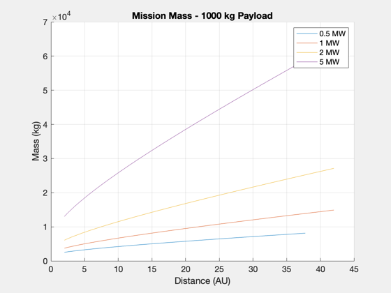
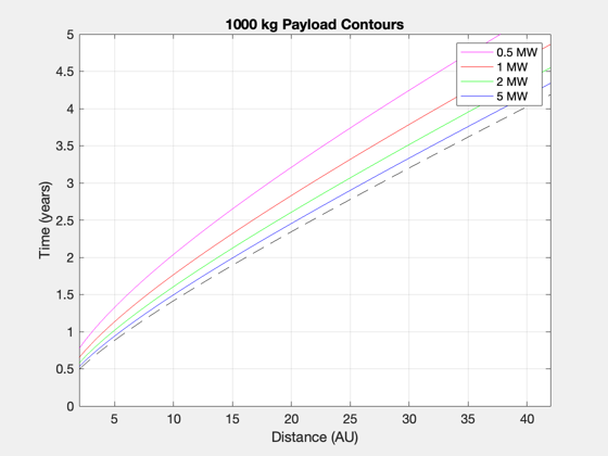
Payload mass contours with power levels

question: how to plot mission mass

h2 = NewFig('Mission Mass'); a2 = axes; hold on; grid on;
NewFig('Payload Contours');
plot(d0s,tFmin/year,'k--'); hold on;  grid on;
mP0 = 1000;
Ps = [0.5 1 2 5]*1e6;
alphas = mP0./Ps;
colors = 'mrgb';
h = [];
for j = 1:length(Ps)
  [c,h(j)] = contour(d0s,tFs,alpha*Ps(j),mP0*[1 1],['-' colors(j)]);
  lambdav = alphas(j) ./ (1/d.sigma + alphas(j) + (1+d.f)*c(2,2:end)*year*2*d.eta/(uE*1e3)^2);
  m0v = mP0./lambdav; % could I plot this on a second y axis?
  plot(a2,c(1,2:end),m0v);
end
xlabel('Distance (AU)')
ylabel('Time (years)')
title('1000 kg Payload Contours')
legend(h,'0.5 MW','1 MW','2 MW','5 MW')
xlabel(a2,'Distance (AU)')
ylabel(a2,'Mass (kg)')
title(a2,'Mission Mass - 1000 kg Payload')
legend(a2,'0.5 MW','1 MW','2 MW','5 MW')

Figui;


%--------------------------------------

% $Id: 42e328e6a2cbbc42da9ba99cc1127f3adbe52a57 $

Published with MATLAB® R2024a