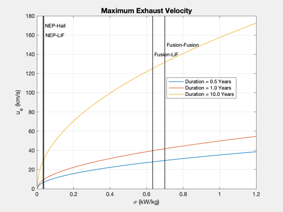
Compute exhaust velocity vs specific power

Generates a plot for several propulsion systems.

See also: Plot2D, SpecificPower

%--------------------------------------------------------------------------

%--------------------------------------------------------------------------
%   Copyright (c) 2018 Princeton Satellite Systems, Inc.
%   All rights reserved.
%--------------------------------------------------------------------------
%   Since 2018.1
%   2019.1 Update fields, exhaust velocity is uE, and sigma in W/kg
%--------------------------------------------------------------------------

eta   = 0.5; % Propulsion efficiency
sigma = linspace(0,1.2)*1000; % Specific power (W/kg)
f     = 0.05; % Fuel tank fraction
sInYr = 86400*365.25;
tau   = [0.5 1 10]*86400*365.25; % Duration
gamma = exp(1); % exp(delta U/uE)
uE    = zeros(length(tau),length(sigma));
leg   = cell(1,length(tau));
for k = 1:length(tau)
  uE(k,:) = sqrt(2*tau(k)*sigma*eta)*sqrt(gamma*f+1-f)./(1+gamma);
  leg{k}  = sprintf('Duration = %2.1f Years',tau(k)/sInYr);
end

[h,hP] = Plot2D(sigma/1000,uE/1000,'\sigma (kW/kg)','u_e (km/s)','Maximum Exhaust Velocity');

pp{1} = 'NEP';
pp{2} = 'Fusion';

en{1,1} = 'Hall';
en{1,2} = 'LiF';

en{2,1} = 'Fusion';
en{2,2} = 'LiF';

sigma = zeros(1,4);

i = 0;
c     = cell(1,4);
for k = 1:2
  for j = 1:2
    i    = i + 1;
    c{i} = sprintf('%s-%s',pp{k},en{k,j});
    sigma(i) = SpecificPower(pp{k},en{k,j});
  end
end

yLim = get(gca,'ylim');

y = yLim(2)-10;
for i = 1:4
	line([sigma(i) sigma(i) ],[0 yLim(2)],'color','k','linewidth',1);
  text(sigma(i)+0.01,y,c{i});
  y = y - 10;
end

legend(hP.h,leg,'location','best')


%--------------------------------------

% $Id: 46de3d5ff5aa96d17063a1dc479d226d56c6554d $

Published with MATLAB® R2024a